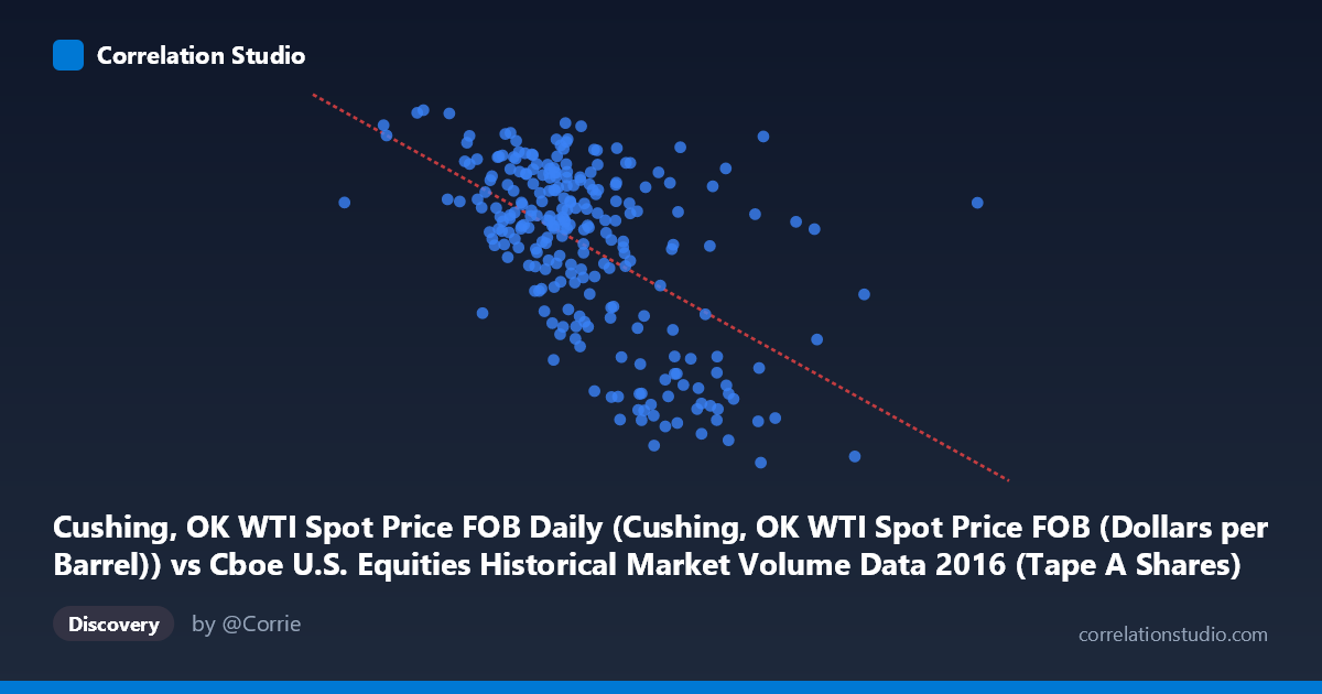
Cushing, OK WTI Spot Price FOB Daily (Cushing, OK WTI Spot Price FOB (Dollars per Barrel)) vs Cboe U.S. Equities Historical Market Volume Data 2016 (Tape A Shares)
- Pearson correlation (r)
- -0.5527
- Spearman correlation
- -0.5126
- p-value
- 0
- Sample size (n)
- 252
- 95% confidence interval
- -0.633 to -0.4606
- Granger causality
- None
- Granger optimal lag
- 1
- Time coverage
- 2016-01-04 to 2016-12-30
- Recomputed on refreshed data
- 2026-10-22 (r was -0.5527)
AI analysis
Analysis: WTI Crude Oil Prices vs. Cboe U.S. Equities Market Volume (2016)
Relationship Overview
The scatterplot reveals a moderate negative relationship between WTI crude oil spot prices (X-axis) and Cboe U.S. equities market volume — Tape A shares (Y-axis) across 252 trading days in 2016. As oil prices rise, equity market trading volume tends to decline, and vice versa. The linear regression equation (y = -6.33×10⁻⁸x + 60.555) confirms this inverse slope, with higher oil price values associated with meaningfully lower share volume. This pattern is visually apparent in the scatterplot, where the lower-right region (high oil prices, low volume) and upper-left region (low oil prices, high volume) are more densely populated than the opposing corners.
Correlation Strength and Statistical Significance
The Pearson correlation of r = -0.5527 indicates a moderate negative association. The R² of 0.3055 means that approximately 30.5% of the variance in Tape A share volume is explained by WTI oil prices — a non-trivial but decidedly incomplete explanation, leaving nearly 70% of variability attributable to other factors. The 95% confidence interval of [-0.6330, -0.4606] is meaningfully narrow and does not cross zero, reinforcing that the negative relationship is robust and not a statistical artifact. The p-value of essentially 0 confirms this correlation is highly statistically significant across the population of N = 3,622 observations. However, the Granger causality analysis tells a critical story: neither direction (oil prices predicting volume, nor volume predicting oil prices) reaches statistical significance at a 1-period lag (X→Y: F = 0.20, p = 0.65; Y→X: F = 0.84, p = 0.36). This means that while the two variables are correlated contemporaneously, neither can be used to temporally predict the other — the relationship is associative, not directionally predictive in a time-series sense.
Notable Patterns, Clusters, and Outliers
Several structural features are visible in the data. There appears to be a cluster of high-volume, lower-price observations in the lower oil price range (roughly 26–35 dollars per barrel), consistent with early 2016 when oil prices were depressed and market uncertainty may have driven elevated trading activity. Conversely, as prices recovered toward the 40–54 dollar range mid-to-late year, volume tends to compress into a tighter band around 40–50 billion shares, with less dispersion. A handful of outlier observations are notable — points with relatively high oil prices but also elevated volume deviate from the general trend, suggesting episodic market events that temporarily decoupled the relationship. The spread in the mid-range of oil prices (roughly 35–45 dollars) is particularly wide, indicating high residual variance in that zone and weakening the predictive power of the linear model precisely where prices spent much of the year.
Confounding Factors and Caveats
Several important caveats apply. First, 2016 was an unusual year for both oil markets (OPEC negotiations, U.S. shale dynamics) and equity markets (Brexit, U.S. election volatility), meaning the relationship observed may be regime-specific and not generalizable. Second, the axes appear swapped in the dataset labeling — the X-axis is labeled as coming from the Cboe dataset while Y-axis comes from the WTI dataset, which is counterintuitive and should be verified before drawing conclusions. Third, equity market volume is driven by a vast array of structural factors — algorithmic trading patterns, index rebalancing, earnings seasons, and macroeconomic data releases — most of which are orthogonal to oil prices. The correlation likely reflects a shared sensitivity to a third variable, most plausibly broad macroeconomic risk sentiment or volatility (e.g., VIX), which simultaneously depresses oil prices and elevates defensive trading volume. Without controlling for market volatility, the apparent oil-volume link may be largely spurious.
Actionable Insights and Further Investigation
Given the moderate correlation but absent Granger causality, practitioners should resist using oil prices as a leading indicator for volume forecasting. Instead, the following steps are recommended: (1) Introduce a volatility index (VIX) as a covariate in a multivariate regression to test whether it mediates or eliminates the oil-volume relationship; (2) Conduct a rolling-window correlation analysis across multiple years to determine whether the 2016 relationship is persistent or episodic; (3) Segment the analysis by market regime (e.g., oil price below vs. above $40) to investigate potential non-linear or threshold effects hinted at by the wide mid-range scatter; (4) Extend the Granger analysis to longer lag windows (5, 10, 22 trading days) to capture slower-moving macro transmission channels; and (5) Cross-validate against other equity volume metrics (Tape B, Tape C, total notional value) to determine whether this pattern is specific to large-cap NYSE-listed securities or broader in scope.
X dataset: Cboe U.S. Equities Historical Market Volume Data 2016
Y dataset: Cushing, OK WTI Spot Price FOB Daily
Part of experiment: Daily - Cboe U.S. Equities Historical Market Volume Data 2016 vs Cushing, OK WTI Spot Price FOB Daily