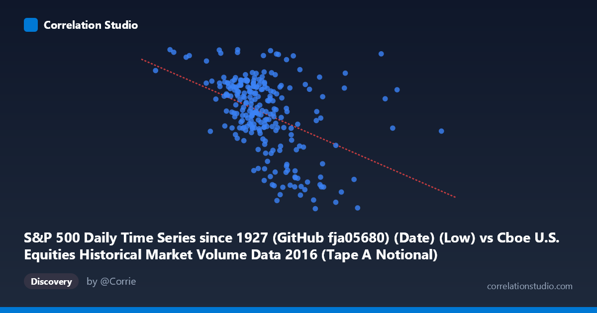
S&P 500 Daily Time Series since 1927 (GitHub fja05680) (Date) (Low) vs Cboe U.S. Equities Historical Market Volume Data 2016 (Tape A Notional)
- Pearson correlation (r)
- -0.4337
- Spearman correlation
- -0.4485
- p-value
- 0
- Sample size (n)
- 252
- 95% confidence interval
- -0.5289 to -0.3276
- Granger causality
- None
- Granger optimal lag
- 1
AI analysis
Scatterplot Analysis: S&P 500 Low vs. Cboe Tape A Notional Volume (2016)
Relationship Overview The scatterplot reveals a negative relationship between the S&P 500 daily low price and Cboe Tape A notional trading volume throughout 2016. As the S&P 500 low price increases (moving right along the x-axis), notional volume tends to decline. This is a broadly intuitive finding in market microstructure: rising equity prices compress the nominal volume of shares needed to achieve equivalent dollar turnover, and calmer bull-market conditions typically generate less urgency-driven trading activity. However, the scatter is visibly wide, and the linear regression (y = -2.58×10⁻⁸x + 2315.54) captures only a modest downward trend amid considerable dispersion.
Correlation Strength and Statistical Significance The Pearson correlation of r = -0.4337 indicates a moderate negative association, but the r² of 0.1881 means that only 18.8% of the variance in Tape A notional volume is explained by the S&P 500 low price level. The remaining ~81% of variance is attributable to other factors entirely. The 95% confidence interval of [-0.5289, -0.3276] is meaningfully narrow and does not cross zero, and the p-value of 5.6×10⁻¹³ confirms the correlation is highly statistically significant — the relationship is real, not a sampling artifact. That said, statistical significance with n=252 drawn from N=3,622 should not be conflated with practical or economic significance; the modest r² tempers enthusiasm considerably. Critically, the Granger causality tests show no significant predictive directionality in either direction (X→Y: p=0.4726; Y→X: p=0.5811), meaning that knowing today's S&P 500 low price does not meaningfully improve next-period forecasts of notional volume, and vice versa. The relationship is contemporaneous and associative rather than temporally predictive.
Notable Patterns, Clusters, and Outliers Several features stand out in the data. There is a dense central cluster roughly between x = 7.5B–10B and y = 2,000–2,200, representing the bulk of "normal" 2016 trading days. A few notable outliers appear at the extremes: points with relatively low S&P 500 lows (circa 7.1–7.6B range on the x-axis) combined with elevated notional volumes approaching 2,250–2,266 likely correspond to the volatile early-2016 sell-off period (January–February), when price levels were depressed but anxious trading drove high volume. Conversely, several points in the upper-right with x 10.5B but y dropping toward 1,850–1,920 suggest the high-price, lower-volume environment of late 2016. One striking point near (6.78B, 2,265) appears as a high-leverage outlier that likely exerts disproportionate influence on the regression slope and deserves scrutiny.
Confounding Factors and Caveats Several confounds complicate a straightforward causal interpretation. Seasonality is a major factor — trading volume follows well-documented intra-year patterns (e.g., summer lulls, year-end effects) that coincide with but are not caused by price levels. The price-level effect on notional value is partly mechanical: if share prices rise, the same number of shares traded produces higher notional value, yet the observed relationship is inverse, suggesting behavioral and structural forces dominate any mechanical effect. The 2016 macro calendar (Brexit in June, U.S. election in November) created episodic volatility spikes that are confounded with both price levels and volume simultaneously. Additionally, Tape A specifically covers NYSE-listed securities, so this is not a full-market measure, and routing behavior between venues can shift notional figures independently of index levels.
Actionable Insights and Further Investigation Despite the modest explanatory power, a few directions merit follow-up. First, segmenting the data by regime (pre/post-Brexit, pre/post-election) would test whether the correlation is driven by a handful of stress episodes rather than a stable structural relationship. Second, controlling for VIX or realized volatility as a covariate would likely absorb much of the residual variance and clarify whether price level has any independent effect on volume beyond volatility's influence. Third, given the failed Granger causality tests, practitioners should not use S&P 500 price levels as a leading indicator for next-day Cboe volume in algorithmic or liquidity-planning models. Finally, extending the analysis across multiple years would establish whether 2016's moderate correlation is representative or anomalous, and whether non-linear models (e.g., piecewise regression around stress thresholds) significantly outperform the current linear fit.
X dataset: Cboe U.S. Equities Historical Market Volume Data 2016
Y dataset: S&P 500 Daily Time Series since 1927 (GitHub fja05680) (Date)
Part of experiment: Daily - Cboe U.S. Equities Historical Market Volume Data 2016 vs S&P 500 Daily Time Series since 1927 (GitHub fja05680) (Date)