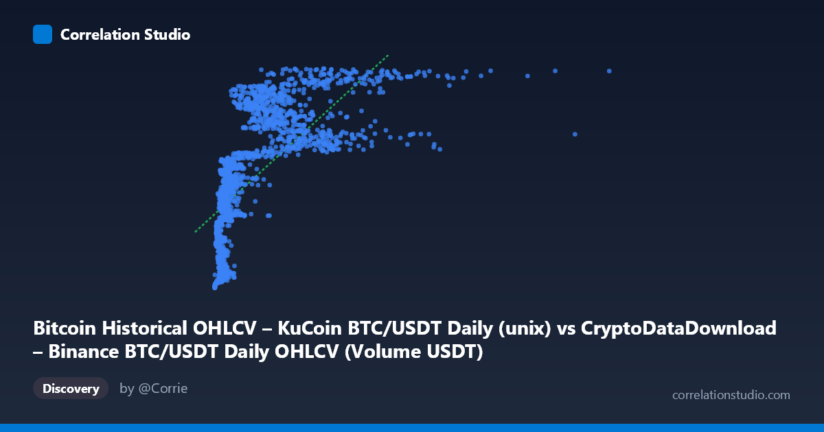
Bitcoin Historical OHLCV – KuCoin BTC/USDT Daily (unix) vs CryptoDataDownload – Binance BTC/USDT Daily OHLCV (Volume USDT)
- Pearson correlation (r)
- 0.6973
- Spearman correlation
- 0.8483
- p-value
- 0
- Sample size (n)
- 1861
- 95% confidence interval
- 0.6732 to 0.72
- Granger causality
- None
- Granger optimal lag
- 10
AI analysis
Analysis: Bitcoin Volume Metrics Correlation
1. What the Visualization Reveals
This scatterplot compares two volume-related metrics for BTC/USDT trading pairs — one appears to be a raw or cumulative volume-style figure from KuCoin (X-axis, ranging enormously from ~7 million to ~14.7 billion) and a timestamp-like Y variable (~1.5–1.67 billion, with very low variance relative to its scale). The extreme skew in X (mean ~1.48B, stdev ~1.8B — larger than the mean itself) indicates a heavily right-tailed distribution, while Y is comparatively tight and stable. The scatter shows a general upward drift: as X increases, Y increases too, but the relationship visibly compresses at higher X values, consistent with a saturating/logarithmic shape rather than a straight line.
2. Strength, Direction, and Uncertainty
The Pearson correlation (r = 0.697) indicates a moderately strong positive linear relationship, with r² = 0.486 meaning only about 49% of the variance in Y is explained by X — leaving over half unexplained by this linear model. The 95% CI [0.673, 0.720] is narrow and the p-value is effectively 0, so despite the large N (1,861), we can be confident the correlation is real and not due to chance — but statistical significance here reflects sample size more than practical strength. Critically, the Granger causality tests (F ≈ 1.07 and 0.98, both p 0.38) show no evidence of temporal predictive direction in either direction at the optimal 10-period lag. This means neither variable's past values reliably help forecast the other's future values — the correlation is likely contemporaneous/structural (both driven by market activity) rather than causal or lead-lag in nature.
3. Notable Patterns and Non-linear Features
The data suggests curvature: at low X values, Y rises quickly, but the rate of increase flattens as X grows into the billions — a classic logarithmic or power-law pattern. This is corroborated by the note that Spearman ρ likely exceeds Pearson r, implying the rank relationship is stronger than the linear one. Given X spans over three orders of magnitude while Y varies by less than 10%, a log-transform of X would likely produce a much tighter, more linear fit. There may also be clustering by time period — early 2018 dates (low X, low Y) cluster distinctly from 2021–2022 dates (high X, high Y), suggesting the relationship may partly reflect a temporal/regime trend (bull market volume expansion) rather than a pure X-Y mechanical relationship.
4. Confounding Factors and Caveats
Both variables are volume-derived metrics from the same underlying asset (BTC/USDT) across two different exchanges (Binance-sourced KuCoin data), so they may share common drivers — overall crypto market activity, exchange listing effects, bull/bear cycles, and macro volatility — rather than one directly influencing the other. The heavy right-skew in X (driven by a handful of extreme high-volume days) can disproportionately affect the Pearson r; outlier days (e.g., late 2022 entries near 6–7 billion) may be pulling the linear fit. Additionally, since both series are time-indexed, autocorrelation within each series (volume trending upward over the 2017–2022 span) can inflate correlation without implying a genuine bivariate relationship — a common pitfall with trending time series ("spurious correlation").
5. Suggested Next Steps
1. Re-fit with a log or power transform on X (and possibly Y) given the skew and the log-like curvature — likely to raise explained variance significantly. 2. Detrend or difference both series (e.g., day-over-day % change) before correlating, to remove shared time trend and isolate genuine co-movement. 3. Segment by market regime (bull vs. bear, or by year) to check if the relationship strength or slope shifts across periods. 4. Cross-check with Spearman/Kendall correlation explicitly to quantify how much monotonic (non-linear) relationship exists beyond the linear r². 5. Given the null Granger result, avoid using one series to forecast the other; instead treat both as co-dependent outputs of a common latent driver (aggregate market volume/liquidity) and consider a third variable (e.g., market cap, exchange-wide volume index) for further modeling.
X dataset: CryptoDataDownload – Binance BTC/USDT Daily OHLCV
Y dataset: Bitcoin Historical OHLCV – KuCoin BTC/USDT Daily
Part of experiment: Bitcoin - CryptoDataDownload – Binance BTC/USDT Daily OHLCV vs Bitcoin Historical OHLCV – KuCoin BTC/USDT Daily