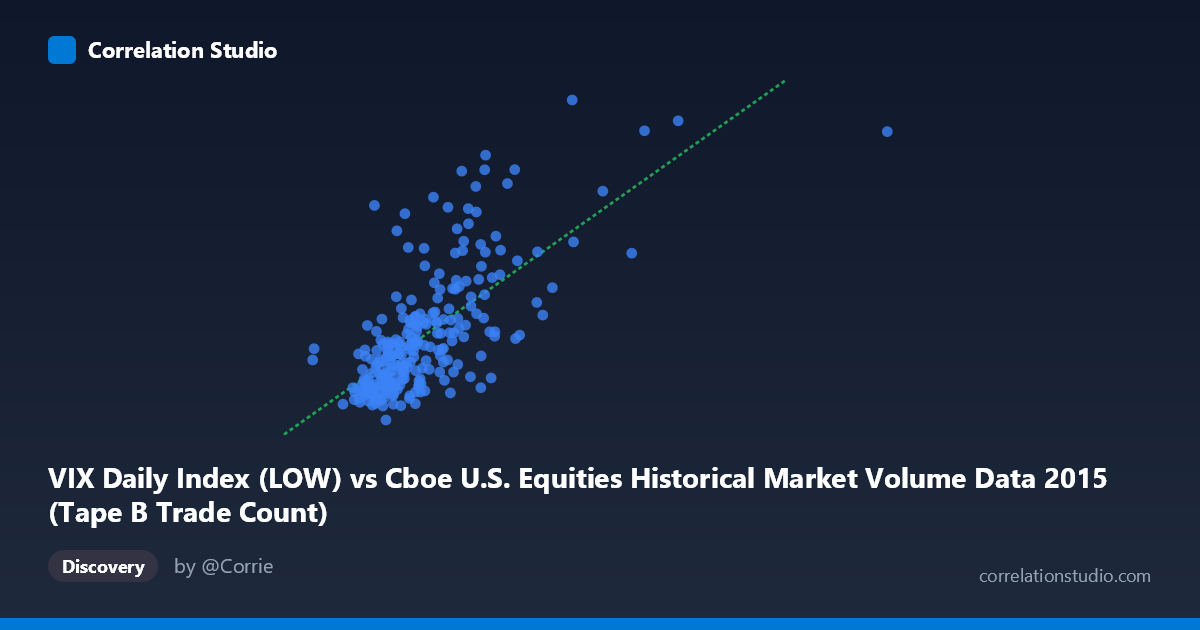
VIX Daily Index (LOW) vs Cboe U.S. Equities Historical Market Volume Data 2015 (Tape B Trade Count)
- Pearson correlation (r)
- 0.6978
- Spearman correlation
- 0.6857
- p-value
- 0
- Sample size (n)
- 252
- 95% confidence interval
- 0.6284 to 0.7561
- Granger causality
- None
- Granger optimal lag
- 1
AI analysis
Analysis: VIX Low vs. Tape B Trade Count (2015)
Relationship Overview The scatterplot reveals a moderately strong positive relationship between the CBOE Volatility Index daily low values (X-axis) and Tape B trade counts (Y-axis) across U.S. equities markets in 2015. As market volume (measured by the VIX low) increases, so too does the number of Tape B trades — a pattern that aligns intuitively with market microstructure theory, where periods of elevated volatility typically drive higher trading activity across exchange segments. The linear regression equation (y = 2.73×10⁻⁵x + 7.68) suggests a modest but consistent positive slope, with the intercept indicating a baseline level of trading activity even at low volume conditions.
Correlation Strength and Statistical Significance The Pearson correlation of r = 0.698 indicates a moderate-to-strong positive association, and the r² of 0.487 means that approximately 48.7% of the variance in Tape B trade counts is explained by VIX low values — a meaningful but far from complete explanation, leaving roughly half the variance attributable to other factors. The 95% confidence interval [0.628, 0.756] is relatively tight, reflecting the substantial sample size (n = 252), and the p-value of essentially zero confirms this relationship is highly unlikely to be a statistical artifact. However, despite this robust contemporaneous correlation, Granger causality tests find no significant temporal predictive relationship in either direction (X→Y: F = 0.132, p = 0.717; Y→X: F = 0.276, p = 0.600). This is a critical nuance: while the two variables move together, neither reliably predicts the other on a lead-lag basis at a one-period lag, suggesting they respond simultaneously to common underlying drivers rather than one causing the other.
Patterns, Clusters, and Outliers The scatterplot shows a concentrated core cluster of observations in the lower-left region (VIX low roughly 130,000–350,000; Tape B counts roughly 11–17), consistent with the relatively calm market conditions that dominated much of early-to-mid 2015. A secondary, more dispersed cluster appears at higher values, reflecting episodic volatility spikes — most notably the August 2015 market correction. Several prominent outliers are visible in the upper-right quadrant, including points near (640,679, 28.08) and (621,009, 20.80), likely corresponding to the late-August volatility surge when VIX spiked dramatically. These outliers exert meaningful leverage on the regression line and may be inflating the overall r value. The relationship also appears to exhibit some heteroscedasticity — variance in Tape B counts increases noticeably at higher VIX low values, suggesting the linear model is a simplification of what may be a more complex, regime-dependent relationship.
Confounding Factors and Caveats Several important caveats warrant caution. First, the axis labels appear potentially swapped in source dataset attribution — the VIX Daily Index column appearing on the X-axis and market volume data on the Y-axis deserves verification, as this could affect interpretive framing. Second, both variables likely share a common driver: broad market stress events (such as the August 2015 correction or end-of-quarter rebalancing) simultaneously elevate volatility and drive trading volume, making the correlation partially spurious in a causal sense. Third, Tape B specifically covers NYSE American (AMEX) and regional exchange listings, meaning it represents a subset of total market activity that may respond differently to volatility than Tape A or C stocks. Seasonal effects, index rebalancing dates, and macroeconomic announcements could also confound the relationship throughout the 2015 calendar year.
Actionable Insights and Further Investigation Practitioners should avoid interpreting this correlation as implying that monitoring VIX lows alone is sufficient for predicting Tape B activity — the unexplained ~51% of variance and absence of Granger causality argue against a simple predictive model. Recommended next steps include: (1) testing a non-linear or piecewise regression model to better capture the apparent regime shift at higher volatility levels; (2) incorporating additional variables such as overall market breadth, VIX high/close values, or macroeconomic event flags to improve predictive power; (3) segmenting the analysis by market regime (calm vs. stressed periods) to assess whether the correlation strengthens meaningfully during volatility episodes; and (4) extending the analysis across multiple years to determine whether the 2015 relationship is structurally stable or driven predominantly by the unique August 2015 volatility event.
X dataset: Cboe U.S. Equities Historical Market Volume Data 2015
Y dataset: VIX Daily Index
Part of experiment: Daily - Cboe U.S. Equities Historical Market Volume Data 2015 vs VIX Daily Index