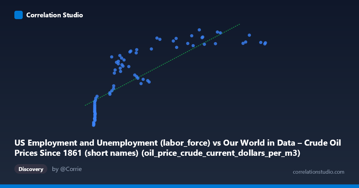
US Employment and Unemployment (labor_force) vs Our World in Data – Crude Oil Prices Since 1861 (short names) (oil_price_crude_current_dollars_per_m3)
- Pearson correlation (r)
- 0.8209
- Spearman correlation
- 0.9172
- p-value
- 0
- Sample size (n)
- 85
- 95% confidence interval
- 0.7367 to 0.8801
- Granger causality
- None
- Granger optimal lag
- 10
- Time coverage
- 1941-01-01 to 2025-01-01
- Recomputed on refreshed data
- 2026-10-09 (r was 0.8166)
AI analysis
Analysis: US Labor Force vs. Crude Oil Prices
1. What the Visualization Reveals
The scatterplot displays a clear positive relationship between annual crude oil prices (in current dollars per cubic meter) and the US labor force size, spanning data from 1941 to 2024. As oil prices rise, so too does the US labor force, and the linear regression line (y = 157.529x + 82,710.7) captures the general upward trend reasonably well. However, the data is far from uniformly distributed — there is a dense cluster of points at very low X values (below ~50), a relatively sparse middle range, and a spread of points at higher oil prices, suggesting the relationship may not be purely linear across its full range.
2. Correlation Strength, Direction, and Causality
The Pearson correlation of r = 0.817 indicates a strong positive association, and R² = 0.667 means that approximately 66.7% of the variance in US labor force size is statistically explained by crude oil prices — a substantial proportion for a two-variable economic model. The 95% confidence interval of [0.730, 0.877] is relatively tight and excludes zero entirely, while the p-value of effectively zero confirms this correlation is highly unlikely to be a sampling artifact. However, the Granger causality results are telling: neither X→Y (F=1.13, p=0.358) nor Y→X (F=1.40, p=0.205) reaches significance, even at a 10-period lag. This means that past oil prices do not meaningfully predict future labor force changes, nor vice versa — the correlation is contemporaneous but not temporally predictive in a causal sense.
3. Notable Patterns, Clusters, and Non-Linearity
The data exhibits several structural features worth noting. A dense cluster of low-X, low-to-moderate-Y points (oil prices below ~50, labor force 53,000–90,000) corresponds to the mid-20th century era of very cheap oil and a smaller workforce. There is then a noticeable gap before points spread across higher oil price ranges with correspondingly larger labor forces. At high X values (above ~400), the Y values appear to plateau between roughly 150,000–168,000, suggesting diminishing returns or saturation in the relationship — the labor force cannot grow indefinitely with rising oil prices alone. A handful of points at extreme X values (699–702) do not yield proportionally higher Y values, hinting at a logarithmic or asymptotic curve that a linear model may be underserving.
4. Confounding Factors and Caveats
The most critical caveat here is that both variables are almost certainly being driven by a common underlying factor: time. The US labor force has grown steadily due to population growth, demographic shifts (particularly female workforce entry), and immigration — trends that are entirely independent of oil prices. Similarly, crude oil prices have trended upward over decades due to depletion, geopolitical dynamics, and inflation. This is a classic spurious correlation driven by shared secular trends, where both series happen to increase over the same historical period. The axis labels also raise a metadata concern: the dataset descriptions appear to have been swapped (labor force data is described under oil prices and vice versa), which warrants verification before drawing any firm conclusions. Additionally, nominal (non-inflation-adjusted) oil prices exaggerate trends compared to real prices.
5. Actionable Insights and Further Investigation
Given the strong correlation but absent Granger causality, the primary recommendation is to detrend both series — for example, by differencing, filtering, or regressing out the time trend — before concluding any meaningful relationship exists. Subsequent steps should include: (1) testing a logarithmic regression model, which may better capture the plateau behavior at high oil prices; (2) examining sector-specific employment (e.g., energy, transportation) rather than total labor force, which may reveal a more direct economic linkage; (3) incorporating inflation-adjusted oil prices to remove the monetary trend component; and (4) exploring breakpoint or regime-change analysis to test whether the oil-price/labor relationship differs meaningfully across eras such as pre-/post-1970s oil shocks or the 2008 financial crisis.
X dataset: Our World in Data – Crude Oil Prices Since 1861 (short names)
Y dataset: US Employment and Unemployment
Part of experiment: Yearly - Our World in Data – Crude Oil Prices Since 1861 (short names) vs US Employment and Unemployment