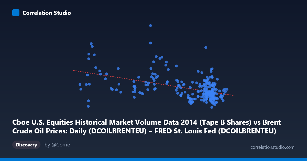
Cboe U.S. Equities Historical Market Volume Data 2014 (Tape B Shares) vs Brent Crude Oil Prices: Daily (DCOILBRENTEU) – FRED St. Louis Fed (DCOILBRENTEU)
- Pearson correlation (r)
- -0.4627
- Spearman correlation
- -0.4186
- p-value
- 0
- Sample size (n)
- 252
- 95% confidence interval
- -0.5545 to -0.3596
- Granger causality
- None
- Granger optimal lag
- 10
AI analysis
Analysis: Brent Crude Oil Price vs. Cboe Tape B Equity Trading Volume (2014)
Relationship Overview The scatterplot reveals a moderate negative relationship between the daily Brent crude oil spot price (X-axis, USD/barrel) and Cboe Tape B equity market trading volume (Y-axis, shares). The linear regression equation (y = −738,857x + 148,310,000) suggests that for every $1 increase in crude oil price per barrel, Tape B equity volume decreases by roughly 738,857 shares on average. Visually, the data points form a broadly descending cloud from left to right, though with considerable scatter, indicating the relationship is real but far from deterministic. The X range spans roughly $55 to $115/barrel — a notably wide band reflecting the oil price decline that characterized much of 2014.
Correlation Strength and Statistical Significance The Pearson correlation of r = −0.463 indicates a moderate negative association, and with r² = 0.214, only 21.4% of the variance in Tape B volume is explained by crude oil price movement. While statistically highly significant (p = 9.1 × 10⁻¹⁵, effectively zero), this leaves nearly 79% of variance unexplained, attributable to other market forces. The 95% confidence interval of [−0.555, −0.360] is reassuringly tight and entirely negative, confirming the direction of the relationship with high confidence given the sample of n = 252 paired observations drawn from a population of N = 3,686. However, statistical significance here is partially a function of sample size — the effect, while real, is modest in practical terms. Critically, Granger causality tests find no significant temporal predictive direction in either direction (X→Y: F = 1.25, p = 0.263; Y→X: F = 1.61, p = 0.104), meaning neither variable meaningfully predicts future values of the other at any tested lag up to 10 periods. This is an important caveat: the correlation is contemporaneous, not predictive.
Notable Patterns, Clusters, and Outliers Several structural features are visible in the data. There appears to be a loose clustering of high-volume observations at lower oil price levels (roughly $55–$75/barrel), consistent with the second half of 2014 when Brent crude fell sharply. Conversely, the bulk of data points at higher oil prices ($100–$115/barrel) show relatively compressed, lower trading volumes. A handful of notable outliers are evident — particularly points near x ≈ 84 and x ≈ 94 with Y values exceeding 160M and 118M shares respectively (e.g., the sample points (84.02, 162,525,288) and (94.57, 118,190,428)), which sit well above the regression line and suggest episodic volume spikes likely tied to specific market events rather than oil price levels. There is also a suggestion of non-linearity or heteroscedasticity: volume variability appears greater at mid-range oil prices than at extremes, which a simple linear model may not fully capture.
Confounding Factors and Caveats Several important caveats apply. First, 2014 was an exceptional year for crude oil — prices were relatively stable around $105–$115 through mid-year before collapsing to ~$55 by year-end, meaning oil price and time are highly collinear. The observed correlation may partly reflect secular intraday or seasonal patterns in equity volume (e.g., year-end volume declines) that happen to coincide with the oil price drop, rather than a causal relationship. Second, Tape B specifically covers regional exchange volume (BATS/EDGA/EDGX), which may respond differently to macro conditions than total market volume. Third, macroeconomic co-movement is a classic confound: both variables could be jointly driven by broader risk-off/risk-on sentiment, USD strength, or geopolitical events (e.g., Middle East tensions, OPEC decisions in late 2014) without directly influencing each other. The absence of Granger causality reinforces that any linkage is likely coincidental or third-variable driven rather than mechanistic.
Actionable Insights and Further Investigation Given the moderate correlation but lack of Granger causality, practitioners should avoid using crude oil prices as a leading indicator for Tape B volume or vice versa. However, the relationship warrants deeper investigation along several lines: (1) Decompose the time series to separate trend from cyclical components — testing whether the correlation persists after removing the shared 2014 downtrend in oil would clarify whether this is a genuine relationship or a spurious trend artifact; (2) Include confounding variables such as VIX (equity volatility), DXY (USD index), and total market volume to build a more complete multivariate model; (3) Test the relationship across multiple years — if the negative correlation only appears in 2014, it strongly suggests a time-specific or coincidental effect; (4) Investigate the high-volume outlier events (e.g., the 162M share day near $84 oil) to identify whether these correspond to identifiable macro events, as they disproportionately influence the regression slope; (5) Consider non-linear or regime-based modeling, as the relationship may behave differently when oil is above versus below $90/barrel.
X dataset: Brent Crude Oil Prices: Daily (DCOILBRENTEU) – FRED St. Louis Fed
Y dataset: Cboe U.S. Equities Historical Market Volume Data 2014
Part of experiment: Daily - Brent Crude Oil Prices: Daily (DCOILBRENTEU) – FRED St. Louis Fed vs Cboe U.S. Equities Historical Market Volume Data 2014