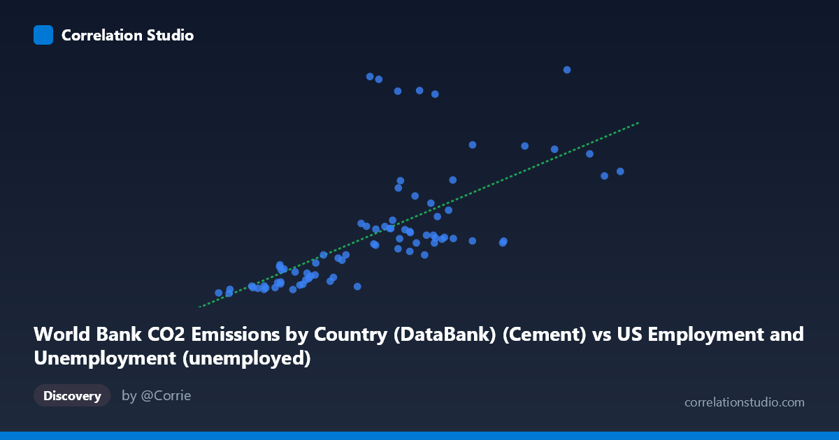
World Bank CO2 Emissions by Country (DataBank) (Cement) vs US Employment and Unemployment (unemployed)
- Pearson correlation (r)
- 0.6683
- Spearman correlation
- 0.812
- p-value
- 0
- Sample size (n)
- 80
- 95% confidence interval
- 0.5258 to 0.7743
- Granger causality
- None
- Granger optimal lag
- 10
- Time coverage
- 1941-01-01 to 2020-01-01
AI analysis
Analysis of World Bank CO2 Cement Emissions vs. US Unemployment
1. Overall Relationship Revealed
The scatterplot reveals a moderate positive association between global CO2 emissions from cement production and US unemployment numbers over the period 1941–2020. As cement-related emissions rise (broadly tracking global industrialization and economic expansion), US unemployment tends to increase in absolute terms as well. However, the scatter is considerable, with many data points deviating substantially from the linear regression line (y = 0.135x − 79.97), suggesting the relationship is far from deterministic and is likely driven by shared underlying trends — most notably, long-run population and economic growth — rather than any direct causal mechanism between the two variables.
2. Correlation Strength, Direction, and Statistical Framing
The Pearson correlation of r = 0.6683 indicates a moderate-to-strong positive linear relationship, but the coefficient of determination r² = 0.4466 means that only 44.7% of the variance in US unemployment is explained by cement CO2 emissions, leaving over 55% attributable to other factors. The 95% confidence interval of [0.5258, 0.7743] is reasonably tight and excludes zero, and the p-value of 1.26 × 10⁻¹¹ confirms the correlation is highly statistically significant — essentially ruling out a chance finding given n = 80. Critically, however, the Granger causality analysis finds no significant predictive directionality in either direction (X→Y: F = 0.874, p = 0.563; Y→X: F = 0.944, p = 0.503) at the optimal lag of 10 periods. This is a key qualifier: even though the variables correlate, neither one temporally predicts the other, strongly suggesting the relationship is spurious co-movement driven by a common third trend rather than any genuine causal pathway.
3. Notable Patterns, Clusters, and Outliers
The data display several visually distinct features worth noting. At lower X values (cement emissions roughly below 4,000 units), unemployment values cluster tightly at low levels, consistent with the mid-20th century period of smaller global industrial output and lower US labor force size. At higher X values, the spread fans out dramatically — a classic heteroscedastic pattern — with several high-leverage outliers visible in the upper range: points such as (12,947; 2,609), (6,314; 2,502), (6,001; 2,533), (7,751; 2,375), and (6,982; 2,368) sit well above the regression line and likely correspond to recession years (e.g., early 1980s, 2009, 2020) when unemployment spiked regardless of emission levels. Importantly, the note that Spearman ρ exceeds Pearson r confirms a non-linear underlying structure, and a logarithmic or polynomial fit would likely explain more variance and reduce the influence of these outliers on model parameters.
4. Confounding Factors and Interpretive Caveats
The most significant caveat is that both variables are strongly trended over time: global cement CO2 emissions have grown nearly monotonically since 1941 alongside industrialization, while US unemployment in absolute numbers (not rate) has grown alongside an expanding labor force. This shared secular trend — essentially a time confound — is the most plausible explanation for the correlation, and the Granger test failure confirms it lacks predictive causal structure. Additionally, US unemployment is driven primarily by domestic business cycle dynamics (recessions, monetary policy, COVID-19 shocks), which have no obvious direct connection to global cement manufacturing activity. The mismatch between dataset labels in the metadata (X-axis labeled as cement data appearing under a US employment dataset, and vice versa) also warrants verification that the data join was performed correctly. Finally, with an optimal lag of 10 periods, the Granger test may be under-powered with only 80 annual observations, reducing confidence in the causality null result.
5. Actionable Insights and Further Investigation
Given these findings, several follow-up analyses are warranted. First, detrending both series (e.g., first-differencing or removing a common time trend) before re-computing correlation would test whether any relationship persists beyond shared growth trajectories. Second, fitting a logarithmic or polynomial regression (as suggested by the Spearman/Pearson discrepancy) could improve model fit and better characterize the non-linear structure. Third, substituting US unemployment rate for absolute unemployment counts would control for labor force growth, potentially collapsing much of the spurious correlation. Fourth, examining recession-year flags as a categorical overlay would help determine whether the high-unemployment outliers cluster around specific economic downturns, clarifying whether the relationship is stable or event-driven. Finally, a partial correlation analysis controlling for year/time would be the most direct test of whether any genuine relationship exists beyond the shared temporal trend.
X dataset: US Employment and Unemployment
Y dataset: World Bank CO2 Emissions by Country (DataBank)
Part of experiment: Yearly - US Employment and Unemployment vs World Bank CO2 Emissions by Country (DataBank)