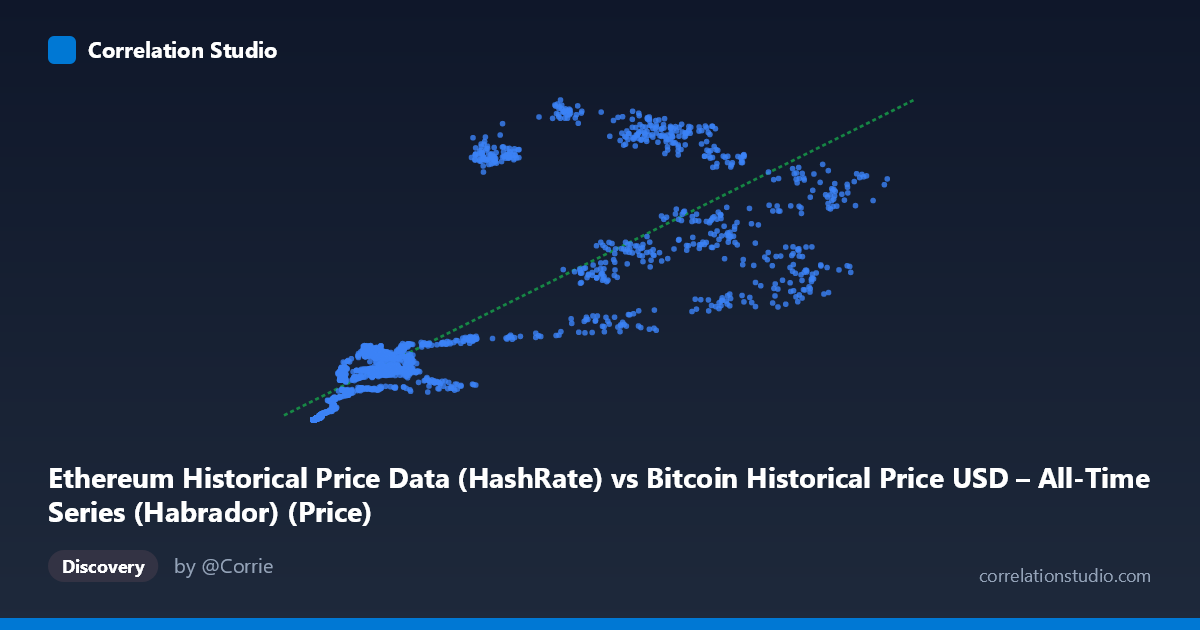
Ethereum Historical Price Data (HashRate) vs Bitcoin Historical Price USD – All-Time Series (Habrador) (Price)
- Pearson correlation (r)
- 0.8175
- Spearman correlation
- 0.91
- p-value
- 0
- Sample size (n)
- 2604
- 95% confidence interval
- 0.8044 to 0.8299
- Granger causality
- None
- Granger optimal lag
- 1
AI analysis
Analysis: Ethereum "HashRate" Field vs. Bitcoin Price Field
(Note: despite the confusing column labels—X is labeled "HashRate" but contains price-scale values, and Y is labeled "Bitcoin Price" but is sourced from an Ethereum dataset—this appears to be a comparison of two cryptocurrency price series, likely Ethereum price on the X-axis and Bitcoin price on the Y-axis, given the value ranges and co-movement.)
1. What the Visualization Reveals
The scatterplot shows a clear positive, roughly linear relationship between the two price series across 2,604 paired daily observations spanning July 2015 to September 2022. As X increases from the low hundreds into the tens of thousands, Y rises correspondingly from near-zero into the hundreds/low thousands range. The data cloud is not a tight line but a broad, upward-trending band, consistent with two assets that generally move together across market cycles but diverge substantially at the day-to-day or event level.
2. Strength, Direction, and Predictive Relationship
The correlation is strong and positive (r = 0.8175, r² = 0.6683), meaning roughly 67% of the variance in Y is statistically explained by X — a substantial but incomplete relationship, leaving about one-third of Y's variance driven by other factors. The 95% CI [0.8044, 0.8299] is tight, and the p-value of ~0 confirms this correlation is highly unlikely due to chance given the large sample (n=2,604). However, correlation strength should not be conflated with causation: the Granger causality tests show no significant predictive direction in either direction (X→Y: p=0.40; Y→X: p=0.31). This indicates that past values of one series do not meaningfully help forecast future values of the other beyond what each series' own history provides — the co-movement is likely driven by a shared external factor (e.g., overall crypto market sentiment, macro liquidity conditions) rather than one asset leading the other.
3. Notable Patterns and Outliers
Several features stand out in the sample data: - Low-end compression: At small X values (< 1,000), Y values are very close to zero (e.g., X=236, Y=0.31; X=452, Y=2.39), suggesting a possible floor effect or early-market period where both assets had minimal, tightly-bound value. - Heteroscedasticity: Variance in Y increases with X. At X≈48,600, Y ranges from 537 to 874 in the sample — a spread of hundreds — while at low X, spreads are only fractions of a point. This fanning-out pattern violates the constant-variance assumption of simple linear regression. - Cycle-related outliers: Points like (20,381, 927) and (29,048, 1,017) sit well above the regression line, while (56,234, 457) sits below it — likely reflecting different bull/bear market phases where the price ratio between the two assets shifted (e.g., "alt season" spikes vs. Bitcoin-dominant phases).
4. Confounding Factors and Caveats
Because both variables are cryptocurrency prices over the same multi-year window, they share obvious macro confounders: overall crypto market cycles, Bitcoin dominance shifts, regulatory news, and broad risk-asset sentiment (e.g., Fed policy, equity market conditions) likely drive both simultaneously. This is a classic case where correlation reflects common exposure to market-wide trends rather than a direct mechanical link. Additionally, time-series data like this are typically autocorrelated (each day's price is close to the prior day's), which inflates apparent correlation and p-values in ways that violate the independence assumptions of standard correlation tests — the "N=3,952 vs n=2,604" discrepancy also suggests missing-data alignment issues that could introduce sampling bias.
5. Suggestions for Further Investigation
To move beyond this surface-level correlation: (1) analyze returns/log-returns rather than raw price levels, which removes trend-driven spurious correlation and better tests genuine co-movement; (2) test for cointegration given both series are likely non-stationary trending series; (3) segment the analysis by market regime (bull/bear/sideways) to see if the relationship strength varies by cycle phase; (4) incorporate a third variable (e.g., a crypto market-cap index or BTC dominance) to test whether it better explains the shared variance, confirming the "common driver" hypothesis over a direct causal one; and (5) clarify the data source/column labeling, as the mismatched dataset names suggest a possible data pipeline error worth resolving before drawing further conclusions.
X dataset: Bitcoin Historical Price USD – All-Time Series (Habrador)
Y dataset: Ethereum Historical Price Data
Part of experiment: Bitcoin - Bitcoin Historical Price USD – All-Time Series (Habrador) vs Ethereum Historical Price Data