Ethereum Historical Data (Daily) (BlkCnt) vs Bitcoin Historical Price USD – All-Time Series (Habrador) (Price)
- Pearson correlation (r)
- 0.6323
- Spearman correlation
- 0.8107
- p-value
- 0
- Sample size (n)
- 3926
- 95% confidence interval
- 0.6131 to 0.6507
- Granger causality
- None
- Granger optimal lag
- 1
- Time coverage
- 2015-07-30 to 2026-04-28
AI analysis
Analysis: Ethereum Block Count vs. Bitcoin Price
1. Relationship Overview
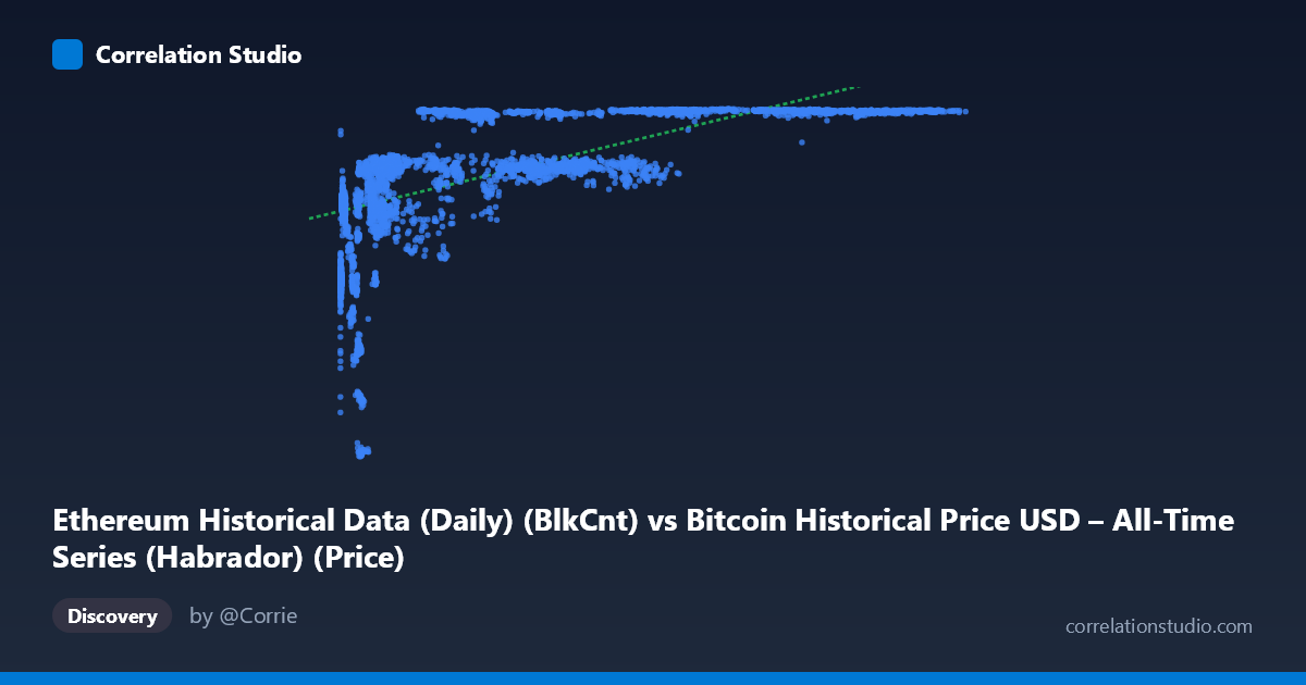
The scatterplot depicts a moderate positive association between Ethereum's daily block count (X) and Bitcoin's USD price (Y). However, the axis labels appear mismatched with the dataset descriptions — the data actually spans two different cryptocurrency metrics that are both proxies for overall crypto market maturity and time. Visually, the relationship is not a clean linear cloud; it resembles a logarithmic or saturating curve: Y rises steeply at low X values, then plateaus into a dense horizontal band (~6,400–7,200) once X exceeds roughly 20,000–30,000. This shape strongly suggests both variables are trending upward over calendar time rather than directly driving one another.
2. Strength, Direction, and Uncertainty
The Pearson correlation (r = 0.632, R² = 0.40) indicates a moderate positive linear relationship, but only 40% of the variance in Y is explained by X — the majority of Y's movement is driven by other factors. The 95% CI [0.613, 0.651] is tight given the large sample (n = 3,926), and the p-value of ~0 confirms the correlation is not due to chance. However, statistical significance here reflects sample size more than practical predictive strength — with R² at only 0.40, this is far from a tight coupling. Critically, the Granger causality tests show no significant predictive direction in either direction (X→Y: p = 0.86; Y→X: p = 0.84). This means neither variable's past values help forecast the other's future values — the correlation is likely contemporaneous/coincidental co-trending (e.g., both rising due to overall market growth over 2015–2026) rather than a causal or lead-lag relationship.
3. Notable Patterns and Non-linearity
The data shows a clear compression/saturation effect: at low X (roughly <10,000), Y ranges widely (2,829–6,500), showing high volatility in early periods. At high X (50,000), Y clusters tightly near its ceiling (7,100–7,200), suggesting Y approaches a resistance level or the dataset's price ceiling within this time window. This pattern — steep rise then flattening — is classic logarithmic growth, consistent with the note that Spearman ρ exceeds Pearson r, confirming a monotonic but non-linear relationship. The linear regression (R² = 0.40) likely underestimates the true monotonic association captured by rank-based methods. A few low-X, low-Y outliers (e.g., X≈2,591–4,630, Y≈3,531–4,686) may represent early market conditions (2015–2016) with structurally different dynamics than later periods.
4. Confounding Factors and Caveats
The most significant caveat is time as a lurking variable: both block count and price plausibly grew over the 2015–2026 window due to network adoption, halving cycles, and broader crypto market bull runs — not because one metric mechanically causes the other. This is a textbook case where spurious correlation via a shared trend can inflate r without genuine causal linkage, reinforced by the null Granger causality results. Additionally, mismatched metadata (column descriptions swapped between X/Y datasets) raises data-integrity concerns that should be resolved before drawing firm conclusions. Structural breaks (halvings, protocol upgrades, market crashes) are not modeled and could distort a simple linear/log fit.
5. Recommendations
1. Refit using a log or logistic model (e.g., Y ~ log(X)) given the clear saturation curve and Spearman/Pearson divergence — this should substantially improve explained variance. 2. Detrend both series (e.g., first-differencing or removing a time trend) before re-testing correlation and Granger causality to isolate any genuine short-term relationship from shared long-term growth. 3. Verify data labeling/alignment — confirm which variable is truly block count vs. price, and ensure timestamps are correctly paired across the two source datasets. 4. Segment by market cycle (bull vs. bear phases, pre/post-halving) to check whether the relationship strength varies by regime, since the pooled correlation may mask regime-dependent effects.
X dataset: Bitcoin Historical Price USD – All-Time Series (Habrador)
Y dataset: Ethereum Historical Data (Daily)
Part of experiment: Bitcoin - Bitcoin Historical Price USD – All-Time Series (Habrador) vs Ethereum Historical Data (Daily)