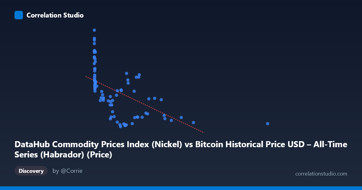
DataHub Commodity Prices Index (Nickel) vs Bitcoin Historical Price USD – All-Time Series (Habrador) (Price)
- Pearson correlation (r)
- -0.5683
- Spearman correlation
- -0.7142
- p-value
- 0
- Sample size (n)
- 83
- 95% confidence interval
- -0.6984 to -0.4018
- Granger causality
- None
- Granger optimal lag
- 10
- Time coverage
- 2010-08-01 to 2017-06-01
- Recomputed on refreshed data
- 2026-10-24 (r was -0.5683)
AI analysis
Analysis: Nickel Price Index vs. Bitcoin Price (USD)
1. Relationship Overview
The scatterplot reveals a moderate negative relationship between the Nickel commodity price index (X) and Bitcoin's historical USD price (Y). As nickel index values increase, Bitcoin prices tend to decrease, though the relationship is clearly not a tight linear band — the data shows substantial scatter, with points clustering heavily at low X values (under ~300) across a wide range of Y values (8,000–28,000), and a sparser tail extending to X≈2452 where Y values compress into the lower range (~9,000–10,000).
2. Strength, Direction, and Uncertainty
The correlation coefficient (r = -0.568) indicates a moderate negative association, with r² = 0.323 meaning only about 32% of the variance in Bitcoin price is statistically explained by nickel index movements — leaving roughly two-thirds unexplained by this single variable. The 95% CI [-0.698, -0.402] is comfortably bounded away from zero, and the p-value (2.1×10⁻⁸) confirms this correlation is highly unlikely to be due to chance in this sample. However, correlation is not causation here: Granger causality tests show no significant predictive direction in either direction (X→Y: p=0.858; Y→X: p=0.532) at the optimal 10-period lag. This strongly suggests the relationship is not one variable temporally driving the other, but rather a spurious or confounded correlation — likely both series independently trending over the 2010–2017 period (e.g., nickel declining during a commodity downturn while Bitcoin experienced its own multi-year growth trajectory) rather than any mechanistic link.
3. Notable Patterns and Outliers
The data shows a clear non-linear, curved pattern rather than a straight-line decline: low-X points (X<50) reach the highest Y values (20,000–28,000), a dense middle cluster (X=100–700) spans nearly the full Y range with high variance, and high-X outliers (X1000, up to 2452) collapse to a narrow low-Y band (~9,000–10,600). This funnel/hyperbolic shape — high variance at low X, low variance at high X — is a hallmark of a logarithmic or power-law relationship, consistent with the note that Spearman ρ exceeds Pearson r. Points near X≈0 with very high Y (e.g., 0.70→28,412; 0.92→26,710) look like extreme leverage points that may be inflating the linear fit's negative slope.
4. Confounding Factors and Caveats
Both series are time-ordered financial/commodity data spanning 2010–2017, a period when Bitcoin underwent enormous secular price appreciation (with cyclical bear/bull swings) while global commodity indices (including nickel) experienced a broad post-2011 downturn. This is a classic case of two non-stationary trending time series producing a spurious correlation — neither may be economically related, but both trend over the same calendar window in opposite directions. Sample size (n=83) is also a subsample of a larger population (N=449), raising questions about how these 83 points were selected/aligned in time, and whether irregular date-matching between two differently-sourced datasets introduces alignment noise.
5. Recommendations
Given the lack of Granger causality, this correlation should not be used for predictive or trading purposes — it's better explained as coincidental trend alignment than a functional economic relationship. Next steps: (1) test detrended or differenced series (returns/changes rather than levels) to check if the relationship persists once shared time trends are removed; (2) fit a log-linear or power model given the funnel-shaped scatter and Spearman/Pearson divergence; (3) investigate a common macro driver (e.g., USD strength, global risk sentiment, Chinese industrial demand) that could simultaneously affect both nickel and speculative asset prices; and (4) expand the sample to the full N=449 population to verify whether the relationship holds at higher resolution.
X dataset: Bitcoin Historical Price USD – All-Time Series (Habrador)
Y dataset: DataHub Commodity Prices Index
Part of experiment: Bitcoin - Bitcoin Historical Price USD – All-Time Series (Habrador) vs DataHub Commodity Prices Index