Cboe U.S. Equities Historical Market Volume Data 2012 (Tape B Shares) vs Bitcoin Historical Price USD – All-Time Series (Habrador) (Price)

Pearson correlation (r): -0.4151
Spearman correlation: -0.3943
p-value: 0
Sample size (n): 250
95% confidence interval: -0.5128 to -0.3069
Granger causality: None
Granger optimal lag: 10
Time coverage: 2012-01-03 to 2012-12-31
Recomputed on refreshed data: 2026-10-24 (r was -0.4151)

AI analysis

Analysis: Cboe Tape B Volume vs. Bitcoin Price (2012)

1. What the Visualization Reveals

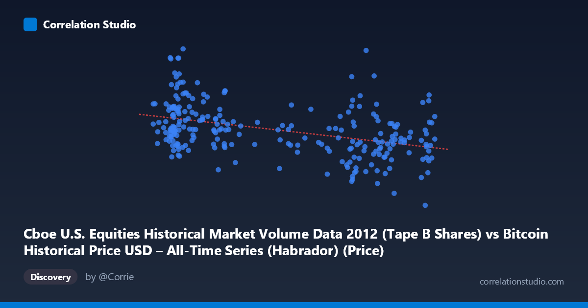
The scatterplot shows a modest negative relationship between U.S. equities market volume (Tape B, Cboe) and Bitcoin's price during 2012. As volume increases along the X-axis, Bitcoin price tends to decline, though the scatter is considerable — points are widely dispersed above and below the regression line rather than hugging it tightly. This is a "loose" negative trend rather than a clean linear relationship.

2. Strength, Direction, and Statistical Confidence

The correlation coefficient (r = -0.415) indicates a weak-to-moderate negative relationship. Critically, r² = 0.172 means only 17.2% of the variance in Bitcoin's price is explained by equity volume — the remaining 82.8% is driven by other factors entirely. While the p-value (7.79 × 10⁻¹²) confirms this correlation is highly statistically significant and not due to chance, and the 95% CI [-0.513, -0.307] confirms the negative direction is robust across the sample, statistical significance here reflects sample size, not practical importance. With n=250, even weak correlations become "significant."

More importantly, the Granger causality tests show no predictive temporal relationship in either direction (X→Y: p=0.547; Y→X: p=0.354). This means past values of equity volume do not help forecast future Bitcoin prices, and vice versa. The correlation is likely contemporaneous/coincidental rather than causal or predictive — a crucial distinction for any forecasting application.

3. Notable Patterns and Outliers

The data clusters into two loose regions: lower X-values (~4-7) paired with higher, more variable Y-values (spanning 27M to 116M), and higher X-values (~10-13) paired with generally lower, tighter Y-values (40M-100M). Several outliers stand out — notably points like (4.86, 110.6M) and (5.75, 97.0M), which sit well above the general trend, and (10.92, 40.5M), which sits below it. The variance in Y appears heteroscedastic: much larger spread at low X than at high X, suggesting the relationship may not be uniform across the range.

4. Confounding Factors and Caveats

This pairing is unusual and warrants caution: Bitcoin price and U.S. equity market volume are governed by largely independent market structures, participants, and macro drivers. Any correlation is more likely a spurious artifact of shared time trends (both series evolving over 2012) rather than genuine market linkage — 2012 Bitcoin was an extremely thin, immature market largely insulated from institutional equity flows. Time-series data like this often exhibits autocorrelation and trending behavior that inflates correlation coefficients without reflecting true dependency (a classic case for spurious regression). Additionally, Bitcoin's own extreme volatility and small market cap in 2012 make it highly sensitive to idiosyncratic shocks unrelated to equities volume.

5. Suggestions for Further Investigation

Given the lack of Granger causality and low r², this relationship should not be used for predictive modeling as-is. Recommended next steps: (a) test for stationarity and detrend both series (e.g., first-differencing) before re-examining correlation, since non-stationary trending data commonly produces misleading r values; (b) explore whether a third variable (overall market liquidity, USD strength, or calendar effects) drives both series independently; (c) consider non-linear or regime-based models given the apparent heteroscedasticity; and (d) treat this pairing primarily as a statistical curiosity unless a plausible economic mechanism linking 2012 Tape B equity volume to Bitcoin pricing can be articulated.

X dataset: Bitcoin Historical Price USD – All-Time Series (Habrador)

Y dataset: Cboe U.S. Equities Historical Market Volume Data 2012

Part of experiment: Bitcoin - Bitcoin Historical Price USD – All-Time Series (Habrador) vs Cboe U.S. Equities Historical Market Volume Data 2012

Scatterplot: Cboe U.S. Equities Historical Market Volume Data 2012 (Tape B Shares) vs Bitcoin Historical Price USD – All-Time Series (Habrador) (Price)