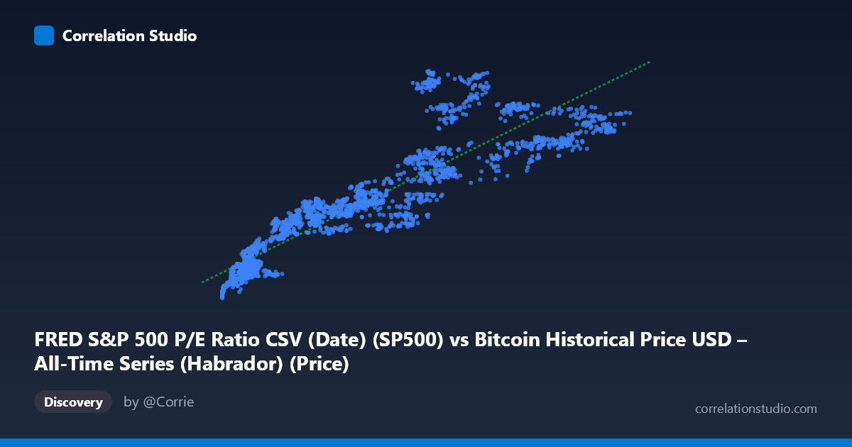
FRED S&P 500 P/E Ratio CSV (Date) (SP500) vs Bitcoin Historical Price USD – All-Time Series (Habrador) (Price)
- Pearson correlation (r)
- 0.9374
- Spearman correlation
- 0.9641
- p-value
- 0
- Sample size (n)
- 2497
- 95% confidence interval
- 0.9324 to 0.942
- Granger causality
- None
- Granger optimal lag
- 10
AI analysis
Analysis: Bitcoin Price vs. S&P 500 P/E Ratio
Note on axis labeling: The axis labels appear swapped in the metadata (X is labeled as "P/E Ratio" but contains values in the thousands to hundred-thousands, consistent with Bitcoin price; Y is labeled "Bitcoin Price" but ranges 2000-7000, consistent with a P/E ratio). The analysis below treats X as Bitcoin price (USD) and Y as S&P 500 P/E ratio, per the actual data ranges.
1. Relationship Overview The scatterplot shows a strong, positive, and visibly curved relationship between Bitcoin price and the S&P 500 P/E ratio. As Bitcoin rises from under $1,000 to over $120,000, the P/E ratio climbs from roughly 2,100 to over 7,000. The sample points suggest a pattern that is monotonic but not strictly linear — the rate of P/E increase appears to slow at higher Bitcoin price levels, hinting at a logarithmic or saturating curve rather than a pure straight line.
2. Strength, Direction, and Statistical Confidence The correlation coefficient (r = 0.937) indicates a very strong positive linear relationship, with R² = 0.879 meaning ~88% of the variance in the P/E ratio is statistically explained by Bitcoin price in this linear model. The tight 95% confidence interval [0.932, 0.942] and p-value of effectively 0 confirm this correlation is highly stable and not due to chance, given the large sample (n=2,497). However, Granger causality tests find no significant predictive direction in either direction (X→Y: p=0.059, borderline; Y→X: p=0.208, not significant). This is a critical caveat: despite the strong contemporaneous correlation, neither variable's past values reliably help forecast the other's future values. This strongly suggests the relationship is driven by a shared underlying trend (e.g., both series rising over calendar time) rather than one variable causing or leading the other.
3. Notable Patterns and Outliers Several features stand out: - Non-linearity: Low-X points (Bitcoin < $10,000) cluster tightly with P/E values in the 2,100–3,400 range, while high-X points (Bitcoin $60,000) show more scatter and steeper P/E values (5,000–7,000), consistent with diminishing marginal effect — a log-linear or power relationship may fit better than the stated linear model. - Time-clustering artifact: Since both series are time series spanning 2016–2026, the correlation likely reflects two independent long-term uptrends (Bitcoin's price appreciation and P/E ratio expansion) that happen to co-occur temporally, not a mechanical linear link. - Possible outliers: A few points (e.g., X≈115,160, Y≈6,345 vs. X≈93,744, Y≈6,902) show inconsistent ordering at the high end, suggesting increased variance/noise at extreme Bitcoin prices — possibly reflecting different market regimes (bull peak vs. correction).
4. Confounding Factors and Caveats This is a spurious correlation risk classic case: both Bitcoin price and equity market P/E ratios have trended upward over the 2016–2026 window due to independent macro forces (loose monetary policy, low rates, retail investor enthusiasm, post-COVID liquidity, AI-driven equity rallies). Neither variable mechanically drives the other; both may be responding to common macro factors (interest rates, risk appetite, liquidity conditions, inflation expectations). The lack of Granger causality reinforces that this is likely a "time trend" confound — correlating any two monotonically increasing series over the same period tends to produce high r values without genuine causal linkage. Additionally, P/E ratios are bounded by earnings dynamics unrelated to crypto markets, so any structural link is implausible on fundamental grounds.
5. Suggestions for Further Investigation - Detrend both series (e.g., first-difference or use returns instead of levels) and recompute correlation — this will reveal whether the relationship survives after removing the shared time trend. It's likely r will drop substantially. - Test against a common third factor, such as 10-year Treasury yields, M2 money supply, or a risk-sentiment index (VIX), to see if both series are driven by shared macro liquidity conditions. - Fit a non-linear model (log-log or log-linear) given the visual curvature, to check if it improves fit over the current linear R² = 0.879. - Treat this correlation as descriptive, not predictive — given the null Granger result, it should not be used for trading signals or forecasting one series from the other.
X dataset: Bitcoin Historical Price USD – All-Time Series (Habrador)
Y dataset: FRED S&P 500 P/E Ratio CSV (Date)
Part of experiment: Bitcoin - Bitcoin Historical Price USD – All-Time Series (Habrador) vs FRED S&P 500 P/E Ratio CSV (Date)