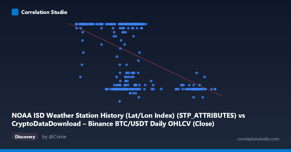
NOAA ISD Weather Station History (Lat/Lon Index) (STP_ATTRIBUTES) vs CryptoDataDownload – Binance BTC/USDT Daily OHLCV (Close)

Pearson correlation (r): -0.4699
Spearman correlation: -0.3046
p-value: 0
Sample size (n): 355
95% confidence interval: -0.5473 to -0.3847
Granger causality: None
Granger optimal lag: 1
Time coverage: 2024-01-01 to 2024-12-31

AI analysis

Scatterplot Analysis: X vs Y Relationship

1. What the Visualization Reveals

The scatterplot shows a moderate negative relationship between the two variables, with Y values clustering heavily near the ceiling (24) across a wide range of X values (roughly 40,000–72,000), then dropping sharply as X extends beyond ~85,000. This creates a pattern that looks less like a classic linear cloud and more like a "shelf-and-drop" structure: Y stays high and saturated for a broad low-to-mid X range, then falls off at high X values. Additionally, within the dense X cluster (40,000–72,000), there is a bimodal split — many points sit at Y=24 while a substantial secondary group sits low (Y=7–12), with relatively few points in between.

2. Strength, Direction, and Statistical Confidence

The correlation coefficient (r = -0.47) indicates a moderate negative linear association, with r² = 0.221 meaning only about 22% of the variance in Y is explained by X — leaving ~78% attributable to other factors or non-linear structure. The 95% CI [-0.547, -0.385] is fairly tight and excludes zero, and the p-value ≈ 0 confirms this relationship is statistically robust and not due to chance, given the large sample (n=355). However, statistical significance here reflects sample size more than practical predictive power — r² of 0.22 is a weak-to-moderate effect size, not one that supports precise point predictions. Critically, the Granger causality tests show no significant predictive direction in either direction (X→Y: p=0.586; Y→X: p=0.266), indicating that despite the cross-sectional correlation, neither variable temporally precedes or predicts the other in a time-series sense. This strongly suggests the correlation is contemporaneous/structural rather than causal.

3. Notable Patterns and Outliers

The most striking feature is the bimodal Y-distribution at moderate X values (40,000–72,000): points split between Y≈24 (ceiling/saturation) and Y≈7-12 (low cluster), with few intermediate values — this is not typical of a smooth linear relationship and suggests either a threshold effect, a mixture of two underlying regimes/subpopulations, or a censored/capped variable (Y maxing at 24 looks like a hard ceiling, possibly hours-in-day or a bounded index). At high X (85,000), Y values consistently collapse to the low range (7-11), driving much of the negative correlation. This suggests the relationship may be driven disproportionately by a smaller subset of high-X observations rather than a uniform trend across the whole range.

4. Confounding Factors and Caveats

Given the dataset labels (BTC/USDT OHLCV vs. NOAA weather station attributes), this pairing is very likely a spurious or mismatched correlation — Bitcoin price/volume data has no plausible causal mechanism linking it to weather station lat/lon attributes. The Granger non-causality result reinforces this: a genuine underlying relationship would typically show at least weak temporal predictability. The apparent correlation may arise from both series independently trending or clustering over the same 2024 time window (e.g., shared time-index artifacts, autocorrelation within each series, or coincidental alignment of value ranges) rather than any real interaction. The Y-ceiling at 24 also hints at a bounded/categorical-like variable (possibly an hour count or station code) that doesn't behave as a continuous linear variable, violating assumptions of simple linear correlation.

5. Recommendations for Further Investigation

Given the likely spurious pairing, the priority should be to verify data provenance and confirm the columns are correctly aligned/labeled — mismatched joins between unrelated datasets (crypto OHLCV and weather station metadata) are a common source of nonsensical "significant" correlations. If the variables are confirmed correct, investigate the bimodal Y clustering with a mixture model or segment the data (e.g., by date, station ID, or X threshold ~75,000) to test whether two distinct regimes explain the split better than one linear fit. A non-linear or piecewise regression (accounting for the ceiling at Y=24) would likely outperform the current linear model. Finally, treat this correlation as descriptive only — the lack of Granger causality and modest r² mean it should not be used for forecasting or causal claims without stronger domain justification.

X dataset: CryptoDataDownload – Binance BTC/USDT Daily OHLCV

Y dataset: NOAA ISD Weather Station History (Lat/Lon Index)

Part of experiment: Bitcoin - CryptoDataDownload – Binance BTC/USDT Daily OHLCV vs NOAA ISD Weather Station History (Lat/Lon Index)