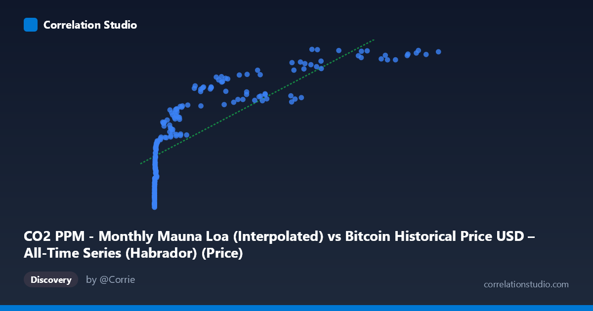
CO2 PPM - Monthly Mauna Loa (Interpolated) vs Bitcoin Historical Price USD – All-Time Series (Habrador) (Price)
- Pearson correlation (r)
- 0.8126
- Spearman correlation
- 0.9725
- p-value
- 0
- Sample size (n)
- 189
- 95% confidence interval
- 0.7578 to 0.8561
- Granger causality
- None
- Granger optimal lag
- 1
AI analysis
Analysis: Bitcoin Price vs. Atmospheric CO2 (Mauna Loa)
1. What the Visualization Reveals
The scatterplot shows a strong positive association between Bitcoin's historical USD price and monthly atmospheric CO2 concentrations, but the shape of this relationship is distinctly non-linear. Data points cluster heavily at low X-values (CO2 readings before Bitcoin's later price surges, or equivalently, Bitcoin prices under ~$1,000) with a long tail extending toward high X-values where Bitcoin prices exceed $50,000–$118,000. This creates a classic logarithmic or power-law curve rather than a straight line — the relationship compresses at high X and stretches at low X, which is exactly the pattern one would expect when combining a monotonically-increasing but nearly-linear geophysical trend (CO2) with an exponentially-growing financial asset (Bitcoin).
2. Strength, Direction, and Statistical Meaning
The Pearson correlation (r = 0.813) is strong and positive, with r² = 0.660 indicating that a linear model explains about 66% of the variance — leaving roughly a third unexplained, which is substantial. The 95% CI [0.758, 0.856] is fairly tight and does not cross zero, and the p-value of 0 confirms this correlation is not due to sampling noise. However, statistical significance here reflects the strength of co-trending over time, not causation — the Granger causality tests confirm this explicitly: neither direction (CO2→Bitcoin: p=0.80; Bitcoin→CO2: p=0.15) shows meaningful predictive power. This is the critical caveat — despite the impressive r², there is no evidence either series temporally "leads" or forecasts the other. The correlation is almost certainly a spurious trend correlation, arising because both series have risen over the 2010–2026 window for entirely unrelated reasons.
3. Notable Patterns and Outliers
- Dense low-X cluster: The majority of points sit below X=10,000 (early Bitcoin history, 2010–2017), where CO2 values ranged narrowly (390–410 ppm) while Bitcoin price varied wildly from $0.06 to a few thousand dollars — this is where most scatter/noise around the trend line occurs. - Sparse high-X tail: Points above X=50,000 (2021+ CO2 readings, corresponding to Bitcoin's bull markets) show CO2 plateauing near 416–429 ppm while Bitcoin price swings between $57,000 and $118,000 — high leverage points that disproportionately anchor the regression slope. - The Spearman Pearson signal: The note that rank correlation exceeds linear correlation confirms the relationship is monotonic but curved — a log-transform of Bitcoin price (or CO2) would likely tighten the fit considerably.
4. Confounding Factors and Caveats
This is a textbook case of two unrelated time trends being correlated purely by shared calendar time. CO2 rises steadily due to fossil fuel emissions; Bitcoin price rose due to adoption cycles, halvings, speculation, and macro liquidity conditions. Both are monotonically increasing over the study window (2010–2026), which mechanically produces high correlation without any causal or mechanistic link. The lack of Granger causality in either direction is the strongest evidence that this is a coincidental trend correlation, not a meaningful relationship. Additionally, mixing a smooth, low-variance natural signal (CO2) with a highly volatile financial asset (Bitcoin, stdev ≈ 29,894 vs. mean ≈ 20,533) means the "relationship" is really just two independent growth curves plotted against each other via a shared time index.
5. Actionable Insights & Further Investigation
- Do not treat this as causal or predictive — the Granger results should be the headline takeaway, not the r² value. - If exploring further, detrend both series (e.g., first-difference or residualize against time) before correlating; genuine co-movement should persist after removing the shared upward trend. Given the near-zero Granger causality, expect the detrended correlation to collapse toward zero. - Try a log-log or log-linear transform (log(Bitcoin price) vs. CO2) to confirm the non-linear fit improves R², but interpret the improved fit only as a better-shaped spurious trend, not stronger causation. - This exercise is a useful illustration of why time-series correlation between unrelated variables requires detrending and causality testing before any real-world claims are made — it's a strong candidate for a "spurious correlation" teaching example (à la Tyler Vigen's website).
X dataset: Bitcoin Historical Price USD – All-Time Series (Habrador)
Y dataset: CO2 PPM - Monthly Mauna Loa
Part of experiment: Bitcoin - Bitcoin Historical Price USD – All-Time Series (Habrador) vs CO2 PPM - Monthly Mauna Loa