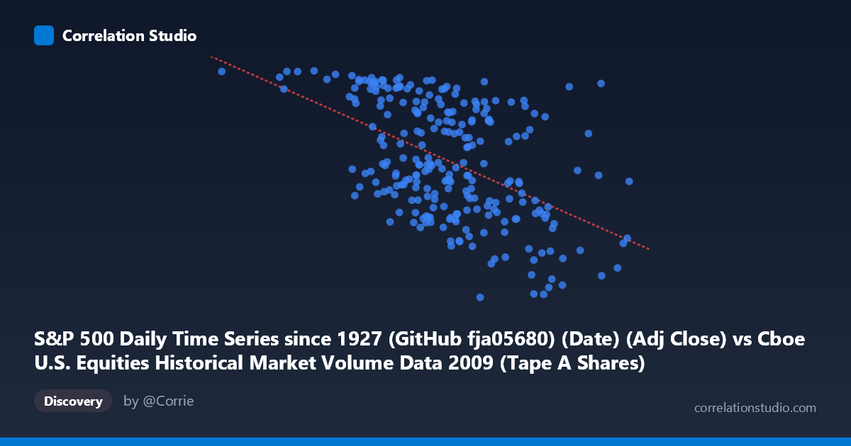
S&P 500 Daily Time Series since 1927 (GitHub fja05680) (Date) (Adj Close) vs Cboe U.S. Equities Historical Market Volume Data 2009 (Tape A Shares)

Pearson correlation (r): -0.5053
Spearman correlation: -0.5003
p-value: 0
Sample size (n): 252
95% confidence interval: -0.5919 to -0.4072
Granger causality: X → Y
Granger optimal lag: 10

AI analysis

Scatterplot Analysis: S&P 500 Adjusted Close vs. Cboe Tape A Shares Volume (2009)

Relationship Overview

The scatterplot reveals a negative relationship between S&P 500 adjusted closing prices (X-axis, representing calendar date as a numeric value mapping to 2009 trading days) and Cboe Tape A shares volume (Y-axis). As the year progresses — from the market's early-2009 lows toward year-end recovery — trading volume in Tape A shares tends to decline. This is visually consistent with the well-documented phenomenon of elevated panic-driven volume during market stress (early 2009 post-crisis) giving way to calmer, lower-volume trading as prices stabilized and recovered through the year.

Correlation Strength and Statistical Significance

The Pearson correlation of r = -0.5053 indicates a moderate negative association, though the coefficient of determination r² = 0.2553 clarifies that only about 25.5% of the variance in Tape A share volume is explained by the S&P 500 price level (date proxy). This means roughly three-quarters of volume variability remains unexplained by this single variable alone. The 95% confidence interval of [-0.5919, -0.4072] is meaningfully distant from zero and entirely negative, lending strong confidence to the direction of the relationship. The p-value of effectively zero confirms this is not a chance finding at any conventional significance threshold. Critically, the Granger causality analysis supports a unidirectional temporal relationship: S&P 500 price movements Granger-cause Tape A volume (F = 2.01, p = 0.033) with an optimal lag of 10 trading periods (~2 weeks), while the reverse direction fails to reach significance (F = 1.15, p = 0.327). This suggests that price signals precede volume changes, not the other way around, at least within this dataset's timeframe.

Notable Patterns, Clusters, and Outliers

The data exhibits considerable vertical scatter at most X values, indicating high volatility in daily volume that is only partially captured by the linear trend. There is a visible high-volume cluster at lower X values (early 2009, approximately X < 300M), corresponding to the crisis-period trough where volume readings approach and exceed 1,100 units — consistent with fear-driven, high-participation trading. Conversely, later in 2009 (X 600M), volume readings cluster more densely in the 700–950 range, with less dispersion. Several notable outliers are visible: points like (662,852,097; 1,102) and (644,338,037; 1,003) appear anomalously high for their late-year position, potentially corresponding to specific event-driven trading days (e.g., earnings seasons, macro announcements). The lower-left corner is relatively sparse, suggesting that even during low-price periods, very low volumes were rare.

Confounding Factors and Caveats

Several important caveats apply. First, the X-axis encodes date as a numeric timestamp, meaning this correlation partly captures a time trend rather than a purely causal price-volume relationship — disentangling date effects from price-level effects requires additional modeling. Second, Tape A volume (NYSE-listed securities) is influenced by many factors beyond the S&P 500 level: algorithmic trading regimes, regulatory changes, options expiration cycles, and index rebalancing events all drive volume independently. Third, 2009 is a structurally unusual year — it spans the final leg of the financial crisis and a dramatic V-shaped recovery — making any correlation from this period potentially non-generalizable to normal market conditions. The Granger result, while statistically significant, uses a modest F-statistic (2.01) that warrants caution about practical predictive power.

Actionable Insights and Further Investigation

Practitioners should explore non-linear models (e.g., piecewise regression or polynomial fits), as the relationship may behave differently in crisis vs. recovery regimes — a regime-switching model segmenting pre- and post-March 2009 trough could be revealing. Given the 10-day Granger lag, a rolling cross-correlation analysis would help determine whether this predictive window is stable across the year or concentrated in specific volatility episodes. Incorporating VIX data as a covariate would help isolate whether fear/uncertainty — rather than price level per se — is the true driver of elevated volume. Finally, extending the analysis to multiple years would test whether this inverse price-volume relationship is a persistent structural feature of U.S. equity markets or an artifact of the 2009 crisis environment.

X dataset: Cboe U.S. Equities Historical Market Volume Data 2009

Y dataset: S&P 500 Daily Time Series since 1927 (GitHub fja05680) (Date)

Part of experiment: Daily - Cboe U.S. Equities Historical Market Volume Data 2009 vs S&P 500 Daily Time Series since 1927 (GitHub fja05680) (Date)