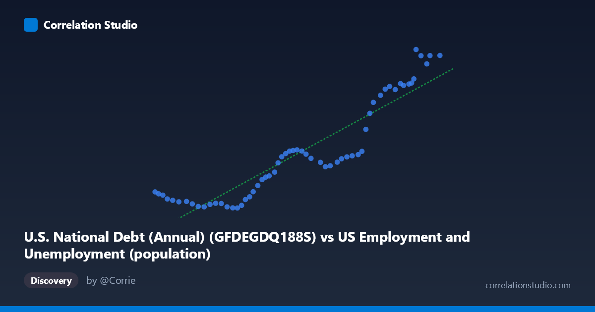
U.S. National Debt (Annual) (GFDEGDQ188S) vs US Employment and Unemployment (population)
- Pearson correlation (r)
- 0.9195
- Spearman correlation
- 0.9178
- p-value
- 0
- Sample size (n)
- 60
- 95% confidence interval
- 0.8684 to 0.9513
- Granger causality
- None
- Granger optimal lag
- 10
AI analysis
Scatterplot Analysis: U.S. National Debt vs. Employment Population
1. Overall Relationship and Visual Pattern
The scatterplot reveals a strong positive relationship between U.S. National Debt (as a percent of GDP) and the U.S. employment population over the period 1966–2025. As the national debt figure increases along the X-axis (ranging from approximately 128,058 to 273,653 in the units provided), the employment population metric on the Y-axis rises correspondingly from roughly 31 to 124. The fitted linear regression line (y = 0.000628x − 63.27) tracks this upward trajectory reasonably well across much of the range, though the scatter around the line is not perfectly uniform, hinting at some structural non-linearity, particularly at the upper and lower extremes of the distribution.
2. Correlation Strength, Direction, and Causal Interpretation
The Pearson correlation of r = 0.9195 indicates a very strong positive association, and the R² of 0.8455 means that approximately 84.6% of the variance in the employment population is statistically explained by variation in the national debt measure within this sample. This is a remarkably high explanatory proportion for macroeconomic data. The 95% confidence interval of [0.8684, 0.9513] is narrow and situated well above zero, and the p-value of effectively 0 confirms that this correlation is highly unlikely to have arisen by chance in a sample of n = 60 paired observations. However, the Granger causality results complicate any causal narrative substantially: neither X→Y (F = 0.7322, p = 0.6887) nor Y→X (F = 1.1928, p = 0.3356) achieves statistical significance at any conventional threshold, even at an optimal lag of 10 periods. This means that, despite the impressively high correlation, neither variable demonstrates meaningful temporal predictive power over the other — past values of national debt do not help forecast future employment population beyond what the employment series itself already predicts, and vice versa. This is a critical finding that strongly cautions against interpreting the correlation as indicative of a direct or lagged causal mechanism.
3. Notable Patterns, Clusters, and Outliers
Examining the data points more closely, several structural features emerge:
- Lower cluster (X ≈ 128,000–175,000; Y ≈ 30–40): Points in this region are tightly grouped near the regression line, suggesting a more stable, predictable relationship during the earlier period when both debt and employment were at lower levels. - Middle zone (X ≈ 175,000–235,000; Y ≈ 40–70): Scatter increases noticeably here. Several points — such as (237,830; 86.51) and (235,801; 77.10) — sit meaningfully above the regression line, while others like (212,577; 57.72) and (217,570; 55.70) cluster closer to or slightly below it. This heteroscedasticity suggests the linear model is less precise in this intermediate range. - Upper cluster (X ≈ 240,000–273,653; Y ≈ 92–124): Points here re-converge toward the regression line and follow a steep, near-linear trajectory. Points like (261,445; 124.04), (273,653; 120.55), and (263,973; 120.40) anchor the upper right, consistent with recent years of simultaneously elevated debt and employment population. No dramatic outliers are visible, though (128,058; 40.34) and (132,028; 38.43) at the lower left appear slightly elevated relative to neighboring X values, potentially reflecting early-period anomalies.
4. Confounding Factors and Interpretive Caveats
Several important caveats must be considered before drawing conclusions from this correlation:
- Shared secular trends (spurious correlation): Both national debt and employment population exhibit long-run upward trends driven by population growth, inflation, GDP expansion, and evolving fiscal policy over six decades. When two time series independently trend upward over time, they will almost always produce high correlations — this is a classic spurious regression problem in macroeconometrics, and the absence of Granger causality strongly reinforces this concern. - Structural breaks: The 1966–2025 window spans multiple distinct fiscal regimes (post-WWII consolidation, Reagan-era expansion, post-2008 crisis debt surge, COVID-19 fiscal response). Each regime may have a different underlying relationship between these variables, and pooling them into a single regression may be misleading. - Reverse causation and third variables: Employment levels affect tax revenues and social spending (and thus debt dynamics), while debt levels may influence economic conditions affecting employment — but both may be primarily driven by a common third factor such as GDP growth, demographic trends, or business cycle phases. - Unit and measurement concerns: The X-axis label describes national debt in what appear to be nominal dollar units, while the Y-axis appears to be population in thousands or similar. The ratio-based nature of debt-to-GDP for one variable versus absolute population for the other creates an implicit scaling dependency that may inflate the apparent correlation.
5. Actionable Insights and Further Investigation
Given the high correlation but absent Granger causality, several investigative steps are warranted:
1. Detrend both series (e.g., using first differences, HP filter, or percentage change transformations) to remove shared secular trends and test whether the correlation persists after controlling for common drift — this is arguably the most important next step. 2. Introduce GDP as a mediating or control variable, since both debt-to-GDP and employment population are downstream of broader economic growth dynamics. A partial correlation or multivariate regression controlling for real GDP would clarify whether the debt–employment relationship is independent or entirely mediated. 3. Test for structural breaks using Chow tests or Bai-Perron methods around known inflection points (2008 financial crisis, 2020 pandemic) to determine whether the correlation is stable or period-specific. 4. Extend the Granger analysis with shorter lag specifications (1–5 periods) and alternative model specifications (VAR with cointegration) to ensure the null finding is robust across methodological choices. 5. Consider policy-relevant sub-period analysis: separating periods of debt-driven fiscal stimulus from periods of passive debt accumulation may reveal heterogeneous relationships with employment outcomes that the aggregate correlation obscures.
In summary, while the statistical association between national debt and employment population is numerically strong, the absence of Granger causality and the presence of likely spurious trending mean this correlation should be treated as a descriptive co-movement artifact rather than evidence of a meaningful directional economic relationship without further rigorous investigation.
X dataset: US Employment and Unemployment
Y dataset: U.S. National Debt (Annual)
Part of experiment: Yearly - US Employment and Unemployment vs U.S. National Debt (Annual)