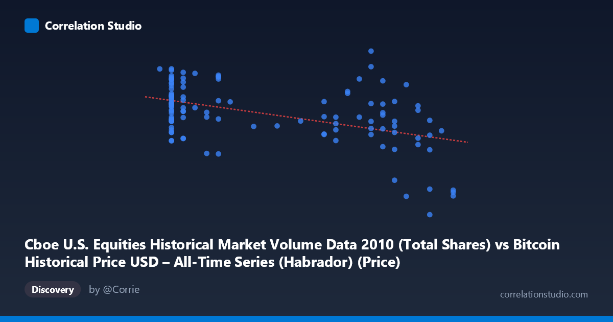
Cboe U.S. Equities Historical Market Volume Data 2010 (Total Shares) vs Bitcoin Historical Price USD – All-Time Series (Habrador) (Price)
- Pearson correlation (r)
- -0.4815
- Spearman correlation
- -0.3954
- p-value
- 0
- Sample size (n)
- 117
- 95% confidence interval
- -0.6097 to -0.3287
- Granger causality
- None
- Granger optimal lag
- 10
AI analysis
Analysis of Cboe Equities Volume vs. Bitcoin Price Relationship
1. What the Visualization Reveals
The scatterplot shows a moderate negative linear relationship between the two variables: as the X variable (labeled here as Cboe equities volume, though the axis definitions appear swapped/mislabeled given the dataset descriptions) increases, Y (Bitcoin price) tends to decrease. The data clusters into a few visible bands—low-X values (0.06–0.11) associated with wide-ranging Y values (roughly 390M–685M), a middle cluster (0.19–0.28) with more moderate Y values, and a distinct low-Y cluster at X≈0.30 (Y around 250–270M). This banding suggests the X variable may be somewhat discretized or that the underlying data has a stepped/categorical quality rather than being purely continuous.
2. Strength, Direction, and Statistical Confidence
The correlation coefficient (r = -0.48) indicates a moderate negative relationship, with r² = 0.232 meaning only 23% of the variance in Y is explained by X — the majority (77%) of variation is driven by other factors entirely. The 95% CI [-0.61, -0.33] is reasonably tight and does not cross zero, and the p-value (3.89E-08) is highly significant, confirming this correlation is not due to chance in this sample. However, statistical significance should not be conflated with practical strength — this is a modest relationship, not a tight predictive one. Critically, the Granger causality tests show no significant predictive direction in either direction (X→Y p=0.30; Y→X p=0.76), meaning that despite the contemporaneous correlation, neither variable helps forecast future values of the other over time. This strongly suggests the relationship is either coincidental, driven by a shared external factor, or purely a static/structural correlation rather than a dynamic causal one.
3. Notable Patterns and Outliers
Several features stand out: (a) a dense cluster at low X (~0.06–0.11) with high variance in Y, ranging from ~395M to ~685M — this cluster alone shows weak internal correlation; (b) a secondary cluster at X≈0.19–0.28 with somewhat lower and tighter Y values; (c) three points at X=0.30 forming a distinct low-Y outlier group (~252–272M), which may be pulling the overall correlation more negative than the bulk of the data would suggest. This suggests the relationship may not be strictly linear — it could be better characterized as flat/noisy across most of the X range with a sharp drop only at the extreme high end.
4. Confounding Factors and Caveats
The axis labeling in the metadata is internally inconsistent (X is described as Cboe volume from a Bitcoin dataset, Y as Bitcoin price from a Cboe dataset), raising concern about a data-merging or labeling error that should be verified before drawing conclusions. Additionally, this covers only a 5.5-month window in 2010 (n=117 of a 3,302-point population), during Bitcoin's very early, thinly-traded, low-liquidity era — price behavior then was dominated by idiosyncratic, low-volume events unlikely to relate meaningfully to modern U.S. equity market structure. Both series likely have their own time-trends (e.g., Bitcoin price drift, seasonal equity volume patterns), and correlating two trending series without detrending can produce spurious correlation.
5. Actionable Recommendations
Before treating this as a meaningful relationship: (1) verify and correct the axis/column labeling to ensure X and Y map to the intended datasets; (2) test for spurious correlation by detrending or differencing both series and re-running the correlation; (3) investigate the X=0.30 outlier cluster separately, as it may be driving a disproportionate share of the negative slope; (4) given the null Granger result, avoid using either series to forecast the other — treat this as a descriptive/contemporaneous association only, not a trading or predictive signal; (5) consider a longer time window or additional covariates (e.g., overall market liquidity, macro events in late 2010) to determine if a third factor better explains both series' movements.
X dataset: Bitcoin Historical Price USD – All-Time Series (Habrador)
Y dataset: Cboe U.S. Equities Historical Market Volume Data 2010
Part of experiment: Bitcoin - Bitcoin Historical Price USD – All-Time Series (Habrador) vs Cboe U.S. Equities Historical Market Volume Data 2010