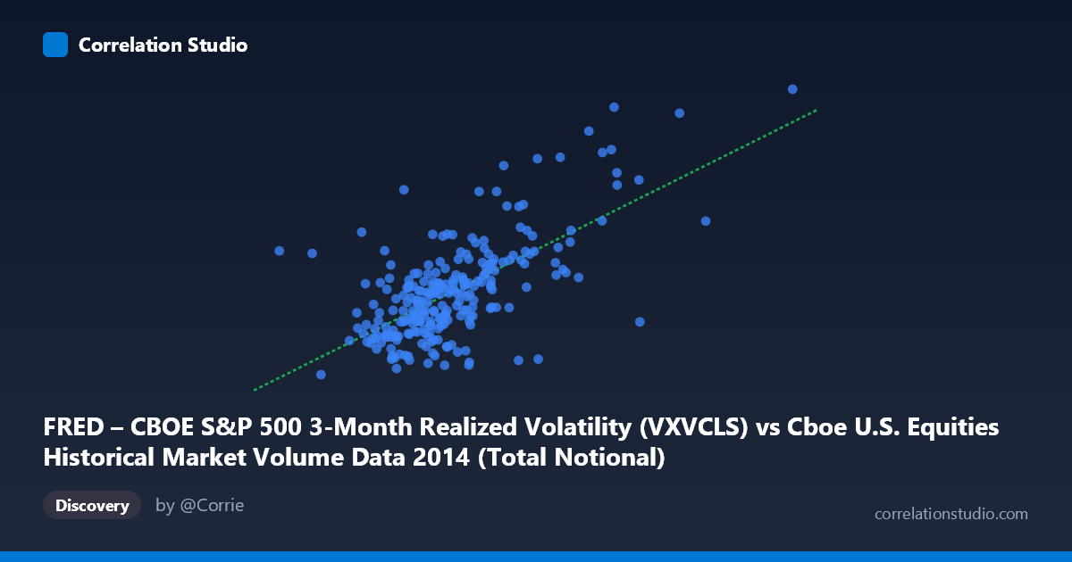
FRED – CBOE S&P 500 3-Month Realized Volatility (VXVCLS) vs Cboe U.S. Equities Historical Market Volume Data 2014 (Total Notional)
- Pearson correlation (r)
- 0.6609
- Spearman correlation
- 0.5712
- p-value
- 0
- Sample size (n)
- 252
- 95% confidence interval
- 0.5851 to 0.7253
- Granger causality
- None
- Granger optimal lag
- 1
AI analysis
Analysis: CBOE S&P 500 3-Month Realized Volatility vs. U.S. Equities Total Notional Volume (2014)
1. Overall Relationship The scatterplot reveals a moderate positive relationship between U.S. equities total notional trading volume (X-axis) and the CBOE S&P 500 3-month realized volatility index (Y-axis) across 252 trading days in 2014. The linear regression equation (y = 3.44×10⁻¹⁰x + 9.47) confirms that as notional volume increases, realized volatility tends to rise as well. This is intuitively consistent with market microstructure theory: elevated trading activity often accompanies — or reflects — periods of heightened uncertainty and price discovery, driving volatility higher. The relationship is visible but clearly imperfect, with substantial scatter around the regression line throughout the range.
2. Correlation Strength and Statistical Significance The Pearson correlation of r = 0.661 indicates a moderate-to-strong positive association, and the R² of 0.437 means that approximately 43.7% of the variance in realized volatility is explained by notional volume — a meaningful but far from complete explanation, leaving over 56% of variance attributable to other factors. The 95% confidence interval of [0.585, 0.725] is reasonably tight and does not approach zero, lending statistical credibility to the finding, and the p-value of effectively zero confirms the result is not a chance artifact given the population size of N = 3,686. However, the Granger causality tests tell an important cautionary story: neither direction (X→Y: F = 2.13, p = 0.145; Y→X: F = 0.36, p = 0.550) achieves significance at conventional thresholds. This means that knowing today's notional volume does not meaningfully improve prediction of tomorrow's volatility, and vice versa — the two variables move together contemporaneously but neither temporally leads the other in a statistically robust way.
3. Notable Patterns, Clusters, and Outliers Several features stand out visually in the data. The bulk of observations cluster in the notional volume range of roughly 13–22 billion, with volatility concentrated between 13 and 18, forming a relatively dense core. However, there are notable high-leverage outliers in the upper-right quadrant — points near (27.3B, 23.09), (31.2B, 22.85), and (24.7B, 17.62) — representing days of extreme volume and elevated volatility, likely coinciding with specific macro events in 2014 (e.g., geopolitical shocks, Fed announcements, or equity selloffs in Q4). Conversely, there are intriguing counter-trend points: (22.9B, 12.87) shows very high volume but unusually low volatility, and (12.5B, 18.02) shows low volume with elevated volatility — both of which deviate meaningfully from the regression line and hint at non-linearity or regime differences. The relationship also appears to fan out (heteroscedastic) at higher volume levels, suggesting the volatility response to volume is less predictable in stressed market conditions.
4. Confounding Factors and Caveats Several important caveats apply. First, 2014 was not a uniform year — it included a sharp equity correction in October driven by Ebola fears and global growth concerns, which likely inflates both volume and volatility simultaneously for a subset of days, potentially overstating the structural relationship. Second, realized volatility is a backward-looking measure (3-month window), meaning any given day's volatility reading reflects conditions from the prior quarter, not just that day — this introduces a temporal mismatch with daily notional volume and may partially explain the absence of Granger causality. Third, notional value is sensitive to price level: in a rising market, the same number of shares traded will register higher notional value, so part of the X-variation may reflect price appreciation rather than genuine volume intensity. Fourth, both variables may be jointly driven by a latent factor — such as macroeconomic uncertainty, institutional rebalancing cycles, or options expiration schedules — making it difficult to assign directional meaning to the correlation alone.
5. Actionable Insights and Further Investigation Despite the absence of Granger causality, the contemporaneous correlation is strong enough to be practically useful. Risk managers and volatility traders could use notional volume as a same-day confirming signal for volatility regime identification, even if it lacks predictive lead-time. For further investigation, it would be valuable to: (1) test non-linear models (e.g., logarithmic or piecewise regression) given the apparent heteroscedasticity and outlier behavior at high volume levels; (2) decompose the analysis by market regime (e.g., pre- vs. post-October correction) to test whether the correlation is structurally stable or event-driven; (3) extend the Granger test to longer lags (beyond the optimal lag of 1) to check for slower-moving predictive dynamics; and (4) incorporate the VIX as a third variable to isolate whether it mediates the volume-volatility relationship, given that VXVCLS is its 3-month companion. Finally, replicating this analysis across multiple years would help determine whether the 2014 findings reflect a durable market mechanism or a sample-specific artifact.
X dataset: Cboe U.S. Equities Historical Market Volume Data 2014
Y dataset: FRED – CBOE S&P 500 3-Month Realized Volatility
Part of experiment: Daily - Cboe U.S. Equities Historical Market Volume Data 2014 vs FRED – CBOE S&P 500 3-Month Realized Volatility