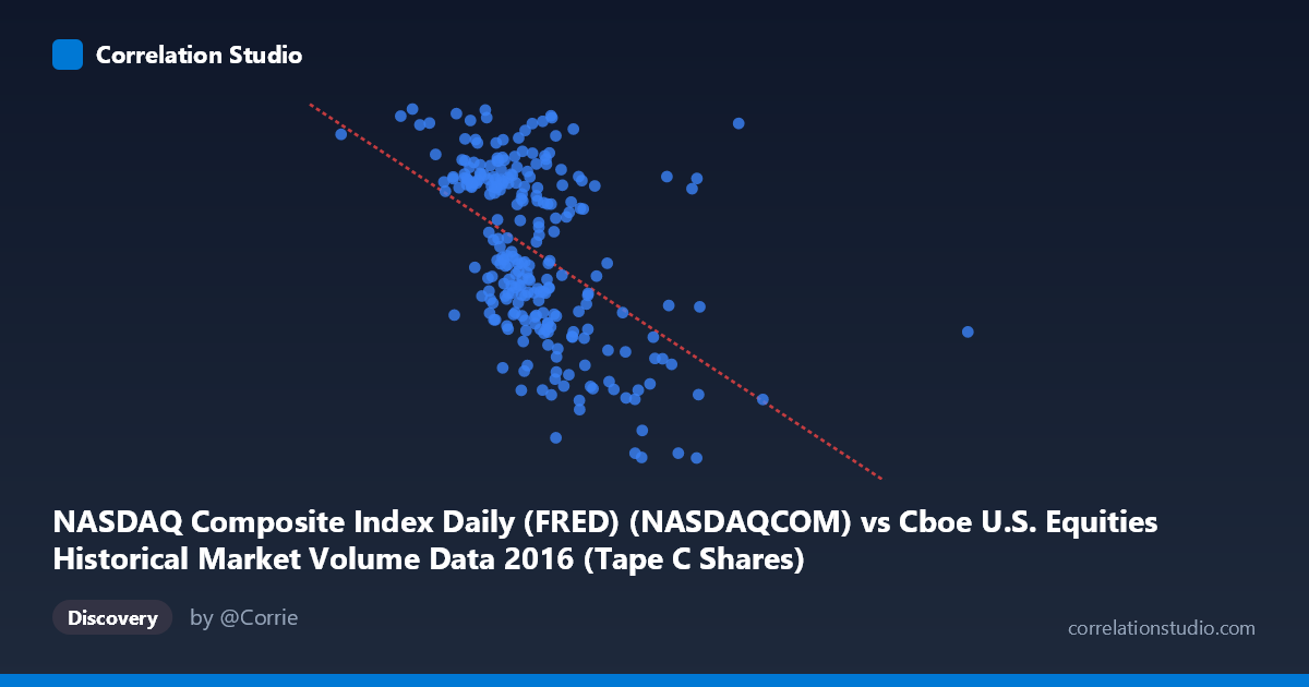
NASDAQ Composite Index Daily (FRED) (NASDAQCOM) vs Cboe U.S. Equities Historical Market Volume Data 2016 (Tape C Shares)
- Pearson correlation (r)
- -0.4988
- Spearman correlation
- -0.5335
- p-value
- 0
- Sample size (n)
- 252
- 95% confidence interval
- -0.5862 to -0.3998
- Granger causality
- None
- Granger optimal lag
- 10
AI analysis
Analysis: NASDAQ Composite Index vs. Cboe U.S. Equities Market Volume (Tape C Shares), 2016
Relationship Overview The scatterplot reveals a moderate negative relationship between daily NASDAQ Composite Index values and Cboe Tape C share volume across 2016. As the NASDAQ index climbed higher, trading volume on Tape C (NYSE Arca-listed securities) tended to decline. This inverse pattern is consistent with a well-documented market phenomenon: during bull market advances, trading activity often contracts as conviction-driven holders reduce turnover, while falling or volatile markets tend to spike volume as participants react defensively or opportunistically.
Correlation Strength and Statistical Significance The Pearson correlation of r = -0.4988 reflects a moderate negative association, and the R² of 0.2488 means that roughly 25% of the variance in Tape C share volume is explained by the NASDAQ index level — leaving approximately 75% attributable to other factors. The 95% confidence interval of [-0.5862, -0.3998] is entirely negative and meaningfully bounded away from zero, reinforcing that the inverse direction is reliable rather than coincidental. The p-value of effectively 0 (against N = 3,622) confirms this relationship is highly statistically significant. However, despite statistical significance, the Granger causality results tell a more cautionary story: neither X→Y (F = 0.5944, p = 0.8177) nor Y→X (F = 0.8334, p = 0.5969) reaches significance at any conventional threshold, even at the optimal 10-period lag. This means that knowing today's NASDAQ level does not meaningfully improve predictions of future Tape C volume beyond its own history, and vice versa. The correlation is contemporaneous and associative, not temporally predictive in either direction.
Notable Patterns and Outliers The sample points reveal several noteworthy features. The bulk of observations cluster in the NASDAQ range of approximately 100M–165M (index values) with Tape C shares between roughly 4,700–5,400, suggesting a dense core relationship. However, there are visible outliers at the lower NASDAQ range (e.g., ~94.5M index, 5,232 shares and ~99.8M index, 5,471 shares) that show elevated volume at lower index levels, consistent with early-2016 market turbulence. At the upper index range (e.g., ~175M, 4,472 shares), volume drops sharply, hinting at possible non-linearity or a threshold effect where the inverse relationship steepens at extreme index values. The linear regression fit (y = -5.44×10⁻⁶x + 5,710.96) captures the general trend, but the wide scatter suggests heteroscedasticity — variance in volume appears larger at lower index levels than higher ones.
Confounding Factors and Caveats Several confounds complicate causal interpretation. Seasonality is a major one: 2016 included distinct volatility episodes (January–February sell-off, Brexit in June, U.S. election in November), each of which simultaneously depressed index levels and spiked volume, mechanically inflating the negative correlation. Mean reversion in volatility could drive both variables without one causing the other. Additionally, Tape C specifically covers NYSE Arca listings, which may behave differently from the broader NASDAQ universe, introducing a compositional mismatch. The dataset represents only a single calendar year (2016), limiting generalizability. Finally, the index level is used here rather than returns — using a trending level variable against a more stationary volume series can introduce spurious correlation, and a more rigorous analysis would employ first-differenced or detrended series.
Actionable Insights and Further Investigation Practitioners and researchers should treat this correlation as descriptive and regime-specific rather than a stable predictive signal. Several follow-up analyses are warranted: (1) Replicate across multiple years to test whether the inverse relationship holds outside 2016's specific volatility regime; (2) Decompose volume by volatility regime (e.g., VIX quartiles) to determine whether the relationship is driven entirely by high-volatility episodes; (3) Use log-transformed or detrended variables to address non-stationarity and potential heteroscedasticity; (4) Extend Granger testing to shorter lags (1–5 periods) to check for very short-term predictive dynamics that the 10-period optimal lag may obscure; and (5) Incorporate additional explanatory variables — such as VIX, bid-ask spreads, or institutional flow data — to better account for the 75% of volume variance left unexplained by the index level alone.
X dataset: Cboe U.S. Equities Historical Market Volume Data 2016
Y dataset: NASDAQ Composite Index Daily (FRED)
Part of experiment: Daily - Cboe U.S. Equities Historical Market Volume Data 2016 vs NASDAQ Composite Index Daily (FRED)