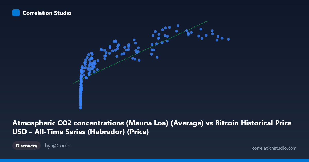
Atmospheric CO2 concentrations (Mauna Loa) (Average) vs Bitcoin Historical Price USD – All-Time Series (Habrador) (Price)
- Pearson correlation (r)
- 0.7993
- Spearman correlation
- 0.9578
- p-value
- 0
- Sample size (n)
- 189
- 95% confidence interval
- 0.7411 to 0.8456
- Granger causality
- None
- Granger optimal lag
- 1
AI analysis
Analysis: Bitcoin Price vs. Atmospheric CO2 Concentration
1. What the Visualization Reveals
This scatterplot pairs Bitcoin's historical USD price against Mauna Loa atmospheric CO2 readings, matched by date. The plot shows a clear upward-sloping pattern: as CO2 concentrations rise (moving left to right through time, since CO2 climbs steadily year over year), Bitcoin's price also trends higher. However, the relationship is heavily compressed at the low end of the X-axis — Bitcoin prices near $390-410 cluster for CO2/X-values under ~1,000, while the dramatic price increases (up to $430) occur only once X exceeds ~20,000-30,000. This creates a curved, logarithmic-looking shape rather than a straight line, which is confirmed by the note that Spearman's rank correlation exceeds Pearson's r.
2. Strength, Direction, and Statistical Meaning
The Pearson correlation (r = 0.79) indicates a strong positive linear association, with r² = 0.629 meaning the linear model explains about 63% of the variance in Y. The 95% CI [0.733, 0.841] is fairly tight and excludes zero, and the p-value (~0) confirms this relationship is statistically robust and not due to chance in this sample. However, statistical significance here is essentially meaningless for causal inference — the Granger causality tests show no predictive direction in either direction (X→Y: p=0.734; Y→X: p=0.108), meaning neither variable helps forecast the other's future movements once past values are accounted for. This is a critical finding: strong correlation with no Granger causality is the hallmark of a spurious relationship driven by a shared trend (both series simply increase over the same calendar period, 2010–2026), not a genuine economic or physical linkage.
3. Notable Patterns and Non-linear Features
The data clearly shows two regimes: a long, flat "low-X" cluster (thousands of points where Bitcoin sat near $390-415 while CO2/X ranged from near-zero to ~10,000) and a sparser "high-X" tail where prices surge toward $420-430. This log-like curvature explains why Spearman's ρ (rank-based, capturing monotonicity) outperforms Pearson's r (linear-only). There are no dramatic outliers breaking the pattern — the shape is consistent with two variables that each grow monotonically over time (CO2 nearly linearly, Bitcoin more like log-linear/exponential with high volatility), rather than genuine point-to-point interaction.
4. Confounding Factors and Caveats
Time is the dominant confound. Both series are independently trending upward over the 2010-2026 window — CO2 due to well-understood emissions accumulation, and Bitcoin due to adoption/speculation cycles. Any two monotonically trending time series will show artificially high correlation purely from shared temporal drift, regardless of any real connection. Additionally, Bitcoin's price is dominated by boom-bust cycles (2013, 2017, 2021 bull runs and subsequent crashes) that have nothing to do with atmospheric chemistry. The mismatched "N vs n" (816 population vs. 187 sampled points) also suggests uneven temporal sampling that could bias the correlation estimate.
5. Actionable Insights and Further Investigation
This correlation should not be interpreted as evidence of any real-world relationship between CO2 levels and Bitcoin prices — it is a textbook example of spurious correlation from co-trending time series. To properly test for any relationship, analysts should: (1) detrend both series (e.g., first-differencing or removing linear/exponential trends) and re-run correlation on the residuals; (2) test cointegration formally rather than relying on Granger causality on levels; and (3) reframe X as "time" explicitly and compare Bitcoin against a true temporal index instead of CO2, since CO2 here is essentially acting as a noisy proxy for calendar date. Given the null Granger results, resources are better spent investigating actual drivers of Bitcoin price (macro liquidity, regulatory events, halving cycles) rather than atmospheric science.
X dataset: Bitcoin Historical Price USD – All-Time Series (Habrador)
Y dataset: Atmospheric CO2 concentrations (Mauna Loa)
Part of experiment: Bitcoin - Bitcoin Historical Price USD – All-Time Series (Habrador) vs Atmospheric CO2 concentrations (Mauna Loa)