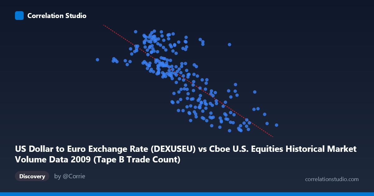
US Dollar to Euro Exchange Rate (DEXUSEU) vs Cboe U.S. Equities Historical Market Volume Data 2009 (Tape B Trade Count)
- Pearson correlation (r)
- -0.7624
- Spearman correlation
- -0.7683
- p-value
- 0
- Sample size (n)
- 250
- 95% confidence interval
- -0.8098 to -0.705
- Granger causality
- None
- Granger optimal lag
- 1
- Time coverage
- 2009-01-02 to 2009-12-31
- Recomputed on refreshed data
- 2026-10-20 (r was -0.7624)
AI analysis
Analysis: USD/Euro Exchange Rate vs. Cboe Tape B Trade Count (2009)
Relationship Overview The scatterplot reveals a moderately strong negative relationship between the US Dollar to Euro exchange rate and Cboe Tape B trade counts during 2009. As the exchange rate increases (dollar strengthening relative to the euro), trade counts tend to decline, and conversely, when the dollar weakens, trading activity is higher. The linear regression equation (y = -4.43425E-07x + 1.57254) captures this inverse trend across the observed range, with the data points forming a discernible downward-sloping cloud rather than a tight line, indicating meaningful but imperfect association.
Correlation Strength and Statistical Significance The Pearson correlation of r = -0.7624 represents a strong negative association, and the R² of 0.5812 indicates that approximately 58% of the variance in Tape B trade counts is statistically explained by variation in the USD/Euro exchange rate — a substantial proportion for financial market data. The 95% confidence interval of [-0.8098, -0.7050] is relatively narrow and entirely negative, confirming consistent directionality with low uncertainty around the estimate. The p-value of essentially zero, across a paired sample of 250 drawn from N = 3,232 observations, makes this correlation highly statistically significant. However, the Granger causality results complicate the narrative considerably: neither direction shows significant predictive causality at conventional thresholds (X→Y: F = 0.0504, p = 0.8225; Y→X: F = 3.0991, p = 0.0796). The marginal Y→X result (p ≈ 0.08) hints that trade counts may weakly lead exchange rate movements, but this falls short of the standard 0.05 threshold. In practical terms, while the correlation is strong, neither variable reliably predicts the other temporally, suggesting the relationship is likely driven by shared external forces rather than direct causation.
Notable Patterns and Outliers The sample points reveal several notable features. The bulk of observations cluster between exchange rates of roughly 280,000–550,000 with trade counts between 1.27 and 1.50, forming the core of the negative trend. There are visible outliers at the extremes: the point at (81,703, 1.44) sits at a very low X value with a mid-range Y, while (766,763, 1.27) represents the highest X value paired with one of the lowest trade counts, consistent with the overall trend. Points like (284,114, 1.50) and (371,276, 1.50) at lower X values with high Y values anchor the upper-left region of the plot. The spread of Y values is notably wider at lower X values (roughly 1.26–1.51) compared to higher X values where Y compresses toward the lower end, suggesting possible heteroscedasticity — variance in trade counts is not uniform across exchange rate levels.
Confounding Factors and Caveats Several important caveats apply. The year 2009 was an extraordinary period in financial markets — the aftermath of the 2008 financial crisis included dramatic swings in both currency valuations and equity trading volumes driven by panic, stimulus responses, and market normalization. Both variables were almost certainly co-driven by macroeconomic stress indicators (VIX, credit spreads, Federal Reserve policy), meaning the observed correlation may be largely spurious — a product of both variables responding to the same crisis dynamics rather than influencing each other. Additionally, the dataset labels appear transposed in the axis descriptions (the X-axis references exchange rate data from a Cboe dataset, and the Y-axis references trade count from an exchange rate dataset), which warrants verification before drawing firm conclusions. The daily lag structure used in Granger testing (lag = 1 period) may also be too short to capture any meaningful temporal dynamics.
Actionable Insights and Further Investigation Given the strong correlation but absence of Granger causality, the most productive next step would be to identify the common driving variable — likely a macro-volatility or risk-appetite measure such as the VIX or credit default swap spreads — and run a partial correlation analysis controlling for it. Researchers should also test longer lag structures (5, 10, 22 trading days) in Granger causality tests to check for delayed predictive relationships. Segmenting the data into early 2009 (crisis recovery phase) versus mid-to-late 2009 (stabilization phase) may reveal whether the correlation is uniform across the year or concentrated in specific volatility regimes. Finally, expanding the analysis to include other exchange rates (USD/GBP, USD/JPY) and other tape classifications (Tape A, Tape C) would help determine whether this pattern reflects a broad currency-equity activity relationship or is specific to this pairing.
X dataset: Cboe U.S. Equities Historical Market Volume Data 2009
Y dataset: US Dollar to Euro Exchange Rate
Part of experiment: Daily - Cboe U.S. Equities Historical Market Volume Data 2009 vs US Dollar to Euro Exchange Rate