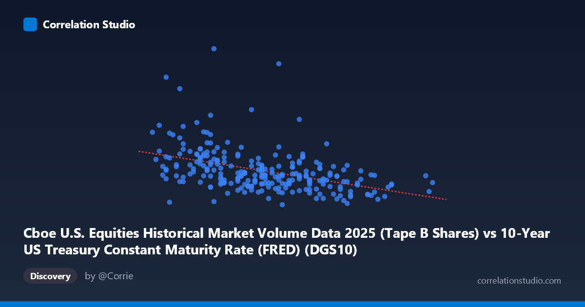
Cboe U.S. Equities Historical Market Volume Data 2025 (Tape B Shares) vs 10-Year US Treasury Constant Maturity Rate (FRED) (DGS10)
- Pearson correlation (r)
- -0.4399
- Spearman correlation
- -0.5088
- p-value
- 0
- Sample size (n)
- 248
- 95% confidence interval
- -0.5352 to -0.3336
- Granger causality
- None
- Granger optimal lag
- 10
AI analysis
Analysis: 10-Year Treasury Yield vs. Cboe Tape B Equity Volume (2025)
Relationship Overview
The scatterplot reveals a moderate negative relationship between the 10-year US Treasury constant maturity rate (x-axis) and Cboe Tape B equity share volume (y-axis) across 248 trading days in 2025. As yields rise, equity market volume on Tape B tends to decline, and the linear regression equation (y = -1.08×10⁸x + 6.29×10⁸) quantifies this: each 1 percentage point increase in the 10-year yield is associated with roughly a 108 million share reduction in daily volume. The data occupies a relatively compressed yield range (3.97–4.79%), yet volume varies enormously — nearly fourfold from ~96M to ~411M shares — suggesting that while yield is a meaningful signal, the relationship is far from deterministic.
Correlation Strength and Statistical Significance
The Pearson correlation of r = -0.44 indicates a moderate negative association, but the explanatory power deserves careful framing: r² = 0.19 means only ~19.4% of the variance in equity volume is explained by Treasury yields, leaving roughly 80% attributable to other forces. The 95% confidence interval of [-0.535, -0.334] is meaningfully away from zero and entirely negative, confirming the direction is reliable. The p-value of 3.68×10⁻¹³ is extraordinarily small, making it statistically unambiguous that this correlation is not a sampling artifact given n = 248. However, Granger causality tests find no significant predictive direction in either direction (X→Y: F = 0.99, p = 0.45; Y→X: F = 0.52, p = 0.87), meaning that past values of Treasury yields do not reliably predict future equity volume, and vice versa. This is a critical distinction: the variables are contemporaneously correlated but neither temporally leads the other, cautioning against any causal or predictive trading interpretation.
Notable Patterns, Clusters, and Outliers
The scatterplot shows a loose, heteroscedastic cloud with greater volume dispersion at lower yield levels (roughly 3.97–4.25%) compared to higher yields. Several prominent outliers stand out: the point near (4.05, 330M) is a substantial upward outlier — approximately 4–5 standard deviations above the conditional mean at that yield — likely corresponding to a specific high-volatility event day such as an index rebalancing, major macro announcement, or market stress episode. Similarly, a cluster of points in the 4.10–4.20% yield range shows extreme volume dispersion (ranging from ~102M to ~243M shares), suggesting that at lower yield environments, idiosyncratic daily factors dominate over the yield signal. At higher yields (4.5–4.7%), volume appears more tightly compressed in the 105M–160M range, hinting at a possible variance-dampening effect at elevated rate regimes.
Confounding Factors and Caveats
Several important caveats apply. First, Tape B specifically captures regional exchange volume (NYSE American, NYSE Arca, etc.), which may respond differently to macro rate signals than consolidated market volume. Second, 2025 represents a single calendar year in a post-hiking-cycle environment, limiting generalizability — the yield range of just 82 basis points compresses the natural variation needed for robust regression inference. Third, seasonal and calendar effects (month-end rebalancing, options expiration weeks, earnings seasons) almost certainly drive much of the unexplained variance and are correlated with neither yield directly. Fourth, the note that dataset column labels appear to be swapped in the axis descriptions (Treasury rate data labeled as volume dataset and vice versa) should be verified before any downstream use. Finally, the contemporaneous nature of the correlation means both variables likely respond to common third factors — risk-off sentiment, Federal Reserve communications, or macroeconomic surprises — rather than one causing the other.
Actionable Insights and Further Investigation
Given the statistically significant but modest correlation and absent Granger causality, practitioners should not use Treasury yields alone as a volume forecasting tool. More productive next steps would include: (1) controlling for VIX or realized volatility, which likely explains a substantial portion of both yield movements and volume spikes simultaneously; (2) decomposing volume by event type (FOMC meeting days, CPI release days, triple-witching) to isolate whether the correlation concentrates on specific macro event windows; (3) testing non-linear specifications (e.g., log-log or piecewise regression) given the apparent heteroscedasticity and the single outlier's outsized influence on the linear fit; and (4) expanding the time series to include multiple rate regimes (2020–2024) to assess whether this negative relationship is structurally stable or specific to the 2025 yield range. The outlier near 330M shares warrants individual date identification as it may represent a regime-changing event disproportionately influencing the regression slope.
X dataset: 10-Year US Treasury Constant Maturity Rate (FRED)
Y dataset: Cboe U.S. Equities Historical Market Volume Data 2025
Part of experiment: Daily - 10-Year US Treasury Constant Maturity Rate (FRED) vs Cboe U.S. Equities Historical Market Volume Data 2025