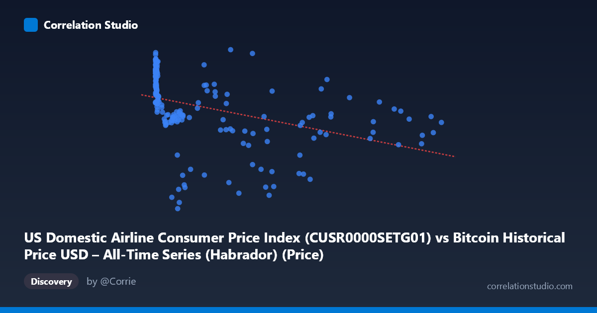
US Domestic Airline Consumer Price Index (CUSR0000SETG01) vs Bitcoin Historical Price USD – All-Time Series (Habrador) (Price)
- Pearson correlation (r)
- -0.4093
- Spearman correlation
- -0.688
- p-value
- 0
- Sample size (n)
- 188
- 95% confidence interval
- -0.5218 to -0.2827
- Granger causality
- None
- Granger optimal lag
- 4
AI analysis
Analysis: Bitcoin Price vs. US Domestic Airline CPI
1. What the Visualization Reveals
This scatterplot pairs Bitcoin's historical USD price (X-axis, spanning an enormous range from $0.06 to $113,500) against the US Domestic Airline Consumer Price Index (Y-axis, ranging 187–325). The data shows a moderate negative trend: as Bitcoin's price climbs into the tens of thousands of dollars, the airline CPI tends to sit lower than during Bitcoin's early, low-price era. However, the relationship is visually noisy — there is no clean, tight linear band, and the sample is dominated by low-value Bitcoin observations (many points cluster near X < 1,000) with a sparser tail of high-price observations.
2. Strength, Direction, and Statistical Meaning
The Pearson correlation is r = -0.41, indicating a moderate negative linear relationship. The r² = 0.168 tells us that only about 16.8% of the variance in airline CPI is statistically associated with Bitcoin price — meaning roughly 83% of airline CPI variation is driven by other factors entirely unrelated to this X variable. The 95% confidence interval [-0.52, -0.28] is reasonably tight and excludes zero, and the p-value (5.5e-9) is highly significant, so we can be confident some real association exists — but "significant" here refers to confidence in the correlation's existence, not its practical strength, which remains modest.
Critically, the Granger causality test shows no significant predictive direction in either direction (X→Y: p=0.067, Y→X: p=0.776). This means neither Bitcoin price nor airline CPI reliably helps forecast the other's future values based on past values. Combined with the modest r², this strongly suggests the correlation is not causal but rather reflects two variables that happen to trend in different directions over the same calendar period — a classic case of spurious correlation driven by shared time trends rather than genuine interaction.
3. Notable Patterns and Non-Linear Features
The note that Spearman ρ exceeds Pearson r is important: it signals the relationship is likely monotonic but non-linear, better captured by a logarithmic or power-law fit than a straight line. This makes sense given Bitcoin's price distribution — it spans nearly 6 orders of magnitude (from $0.06 to $113,500), so a linear model is poorly suited; small-dollar-value points dominate the scatter while high-price points (Bitcoin bull-run peaks) are few but highly leveraged in the regression. Visually, the low-X cluster (Bitcoin under ~$1,000) shows CPI values spread across almost the entire Y range (280–320), while high-X points (Bitcoin above $50,000) tend to cluster in a lower/mixed CPI band (215–290), suggesting the "signal" is concentrated in distinguishing early vs. late Bitcoin eras rather than a smooth continuous relationship.
4. Confounding Factors and Caveats
The most obvious confound is time itself. Bitcoin price has grown roughly exponentially since 2010, while airline CPI has evolved due to its own drivers (fuel costs, COVID-19 collapse and recovery, seasonal demand, airline industry consolidation). Both series are non-stationary time series that trend over a shared 2010–2026 window; correlating two trending series without differencing or detrending very commonly produces artificially significant correlations. The mismatched, highly skewed X distribution (mean $20,011 vs. median likely far lower) also means a handful of extreme Bitcoin values could disproportionately influence the linear fit. Additionally, comparing a monthly CPI index to Bitcoin's famously volatile, near-continuous price series introduces temporal alignment/aggregation issues (e.g., which Bitcoin price observation is paired with which month's CPI reading).
5. Suggestions for Further Investigation
Given the lack of Granger causality and the likely spurious nature of this trend-driven correlation, analysts should: (1) detrend or difference both series (e.g., use month-over-month % changes) and recompute correlation to test if the relationship survives — it likely will weaken substantially; (2) apply a log transform to Bitcoin price given its exponential growth and multi-order-of-magnitude range, then retest linear correlation; (3) explore third-variable confounders like macroeconomic conditions (inflation, interest rates, fuel prices, COVID-era demand shocks) that could independently drive both series; and (4) treat this correlation as descriptive/coincidental rather than a basis for any predictive or trading strategy, given both the weak r² and the absence of Granger-causal predictive power in either direction.
X dataset: Bitcoin Historical Price USD – All-Time Series (Habrador)
Y dataset: US Domestic Airline Consumer Price Index
Part of experiment: Bitcoin - Bitcoin Historical Price USD – All-Time Series (Habrador) vs US Domestic Airline Consumer Price Index