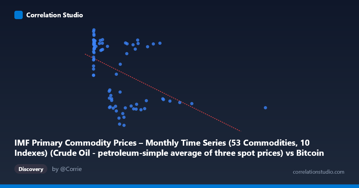
IMF Primary Commodity Prices – Monthly Time Series (53 Commodities, 10 Indexes) (Crude Oil - petroleum-simple average of three spot prices) vs Bitcoin Historical Price USD – All-Time Series (Habrador) (Price)
- Pearson correlation (r)
- -0.4787
- Spearman correlation
- -0.4701
- p-value
- 0.000005
- Sample size (n)
- 83
- 95% confidence interval
- -0.6294 to -0.2933
- Granger causality
- None
- Granger optimal lag
- 1
- Time coverage
- 2010-08-01 to 2017-06-01
AI analysis
Analysis: Bitcoin Price vs. Crude Oil Price
1. What the Visualization Reveals
The scatterplot shows a moderate negative relationship between crude oil prices (X-axis) and Bitcoin prices (Y-axis) across this 2010–2017 sample. The data is heavily skewed toward low oil prices (most points cluster below $700, with the mean at $321 but a max of $2,452), while Bitcoin prices show a more bimodal spread — a dense cluster near $95–118 (low X values) and another cluster near $29–55 (higher X values). This creates the visual impression of an inverse relationship, but it's driven largely by two distinct regimes rather than a smooth linear trend.
2. Strength, Direction, and Statistical Confidence
The correlation coefficient (r = -0.479) indicates a moderate negative relationship, with r² = 0.229 meaning only ~23% of the variance in Bitcoin price is explained by oil price — leaving roughly 77% attributable to other factors. The 95% CI [-0.629, -0.293] is reasonably tight and entirely negative, and the p-value (4.7×10⁻⁶) is highly significant, so we can be confident a real (non-zero) negative association exists in this sample. However, statistical significance should not be conflated with practical predictive power — with only 23% variance explained, oil price alone is a weak predictor of Bitcoin price. Critically, the Granger causality tests show no significant temporal predictive direction (X→Y: p=0.16; Y→X: p=0.18), meaning neither series reliably "leads" the other at a 1-period lag. This suggests the correlation is likely coincidental co-movement (or driven by a shared underlying trend) rather than one variable causally driving the other.
3. Notable Patterns and Outliers
The most striking feature is the clustering structure: a dense group of ~30 points with very low X (near $0–35) and high Y (~90–118) represents Bitcoin's earliest, pre-2013 era when oil was scraping historic lows and Bitcoin was newly emergent and volatile. A second cluster sits at moderate X (200–650) with lower Y (~30–65), and a sparse tail of high-X outliers (oil $700, up to $2,452) with Y around 45–105. This is not a continuous linear relationship but more like distinct time-period clusters — suggesting the apparent correlation may be an artifact of both variables trending over the sample period rather than a direct functional relationship.
4. Confounding Factors and Caveats
Both series are time-ordered and non-stationary — Bitcoin's price grew from cents to significant values over this window, and oil prices also experienced major regime shifts (2014-2016 crash). Correlating two trending time series often produces spurious correlation unrelated to any causal mechanism (a classic "trending confound"). Additionally, small sample size (n=83, likely monthly aggregates over ~7 years) limits granularity, and the extreme skew in X (max 2452 vs. mean 321) means a few outliers could disproportionately influence the fitted regression line. Macroeconomic factors (USD strength, global risk sentiment, monetary policy) likely drive both series independently.
5. Suggestions for Further Investigation
Given the non-stationarity concern, analysts should difference or detrend both series (e.g., use % changes or log returns rather than levels) and re-run correlation/Granger tests — this often eliminates spurious level-correlations. Additionally, segmenting the analysis by distinct market regimes (pre-2013 vs. 2013-2017) could clarify whether the relationship is regime-dependent or an artifact of pooling structurally different periods. Finally, given the lack of Granger causality, treat this correlation as descriptive, not predictive — it should not be used for trading signals or forecasting without further validation using more granular, stationarity-adjusted data.
X dataset: Bitcoin Historical Price USD – All-Time Series (Habrador)
Y dataset: IMF Primary Commodity Prices – Monthly Time Series (53 Commodities, 10 Indexes)
Part of experiment: Bitcoin - Bitcoin Historical Price USD – All-Time Series (Habrador) vs IMF Primary Commodity Prices – Monthly Time Series (53 Commodities, 10 Indexes)