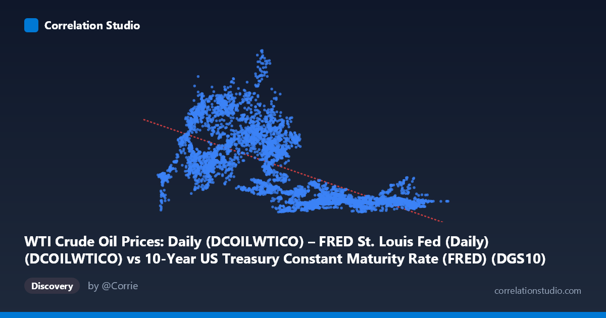
WTI Crude Oil Prices: Daily (DCOILWTICO) – FRED St. Louis Fed (Daily) (DCOILWTICO) vs 10-Year US Treasury Constant Maturity Rate (FRED) (DGS10)
- Pearson correlation (r)
- -0.6588
- Spearman correlation
- -0.7105
- p-value
- 0
- Sample size (n)
- 10058
- 95% confidence interval
- -0.6697 to -0.6476
- Granger causality
- None
- Granger optimal lag
- 1
AI analysis
WTI Crude Oil Prices vs. 10-Year US Treasury Yield: Correlation Analysis
Relationship Overview
The scatterplot reveals a moderate negative relationship between WTI crude oil prices (X-axis) and the 10-year US Treasury constant maturity rate (Y-axis), spanning nearly four decades of daily data from 1986 to 2026. The linear regression equation (y = -8.59x + 88.17) indicates that for every $1 increase in WTI oil prices, the 10-year Treasury yield tends to decrease by approximately 8.59 basis points — a counterintuitive pattern at first glance, but one that reflects the complex macroeconomic regimes captured across this long time horizon. The scatter of points is notably wide, suggesting that while the trend is real, many individual observations deviate substantially from the regression line, hinting at structural breaks and regime-dependent behavior across different economic eras.
Correlation Strength and Statistical Significance
The correlation coefficient of r = -0.6588 indicates a moderate-to-strong negative association, but the explanatory power is more sobering: R² = 0.434 means only 43.4% of the variance in Treasury yields is explained by oil prices, leaving the majority of variation unaccounted for by this single variable. The 95% confidence interval of [-0.6697, -0.6476] is exceptionally narrow, and the p-value is effectively zero — both attributable to the very large paired sample size (n = 10,058), which means the correlation is estimated with high precision and is unambiguously statistically significant. However, statistical significance here must not be conflated with practical or causal significance. Crucially, the Granger causality tests find no significant predictive directionality in either direction (X→Y: F = 2.22, p = 0.14; Y→X: F = 0.01, p = 0.90), meaning that neither variable's past values meaningfully predict the other's future values at the tested lag. This firmly cautions against any causal interpretation: the correlation is a structural association, not a temporal forecasting signal.
Notable Patterns, Clusters, and Outliers
Examining the sample points reveals several striking features. There is a visible cluster of low-oil-price, high-yield observations (e.g., oil ~1–3, yields ~75–110), which likely corresponds to the late 1980s through 1990s when Treasury yields were elevated and oil was relatively cheap. Conversely, high-oil-price observations tend to cluster at low yield values (e.g., oil ~7–10, yields ~10–25), consistent with the post-2008 era of quantitative easing and suppressed interest rates coinciding with elevated oil demand periods. Several outliers are apparent — for instance, a point at (3.25, 109.56) represents a period of very low oil prices and extremely high yields, anchoring the upper-left region of the chart. The scatter is heteroscedastic: dispersion in Y is much wider at low X values, suggesting the relationship is not uniformly linear and may better reflect two or three distinct macroeconomic regimes rather than a single continuous relationship.
Confounding Factors and Caveats
This correlation is almost certainly driven by shared historical time trends rather than a direct economic mechanism. Both variables are heavily influenced by common macro forces — Federal Reserve monetary policy cycles, inflation regimes, global growth conditions, geopolitical events, and energy market structural shifts — that evolved dramatically across 1986–2026. The long time horizon conflates multiple distinct eras: high-rate/low-oil 1980s–90s, low-rate/high-oil 2000s commodity boom, the post-GFC zero-lower-bound period, the COVID shock, and the 2022 inflation surge. Each epoch represents a different structural relationship. Treating this as a stable bivariate relationship risks spurious correlation driven by coincident secular trends rather than any meaningful economic linkage. Additionally, axis labeling in the metadata appears swapped (WTI is plotted on X, yields on Y), which should be verified before drawing directional conclusions.
Actionable Insights and Further Investigation
Given the absence of Granger causality, this correlation should not be used for short-term forecasting or trading signals. However, several productive follow-up analyses are warranted. First, regime-segmented analysis — splitting the data into distinct monetary policy eras (pre-2000, 2000–2008, 2009–2021, 2022–present) — would likely reveal very different within-regime correlations and help disentangle structural from spurious effects. Second, multivariate modeling incorporating inflation expectations (TIPS breakevens), Fed Funds rate, and USD index would sharply reduce the unexplained 56.6% of variance. Third, testing non-linear specifications (polynomial or piecewise regression) may better capture the apparent heteroscedasticity. Finally, cointegration testing over the full time series would determine whether any long-run equilibrium relationship exists, which would be more economically meaningful than the contemporaneous correlation alone.
X dataset: 10-Year US Treasury Constant Maturity Rate (FRED)
Y dataset: WTI Crude Oil Prices: Daily (DCOILWTICO) – FRED St. Louis Fed (Daily)
Part of experiment: Daily - 10-Year US Treasury Constant Maturity Rate (FRED) vs WTI Crude Oil Prices: Daily (DCOILWTICO) – FRED St. Louis Fed (Daily)