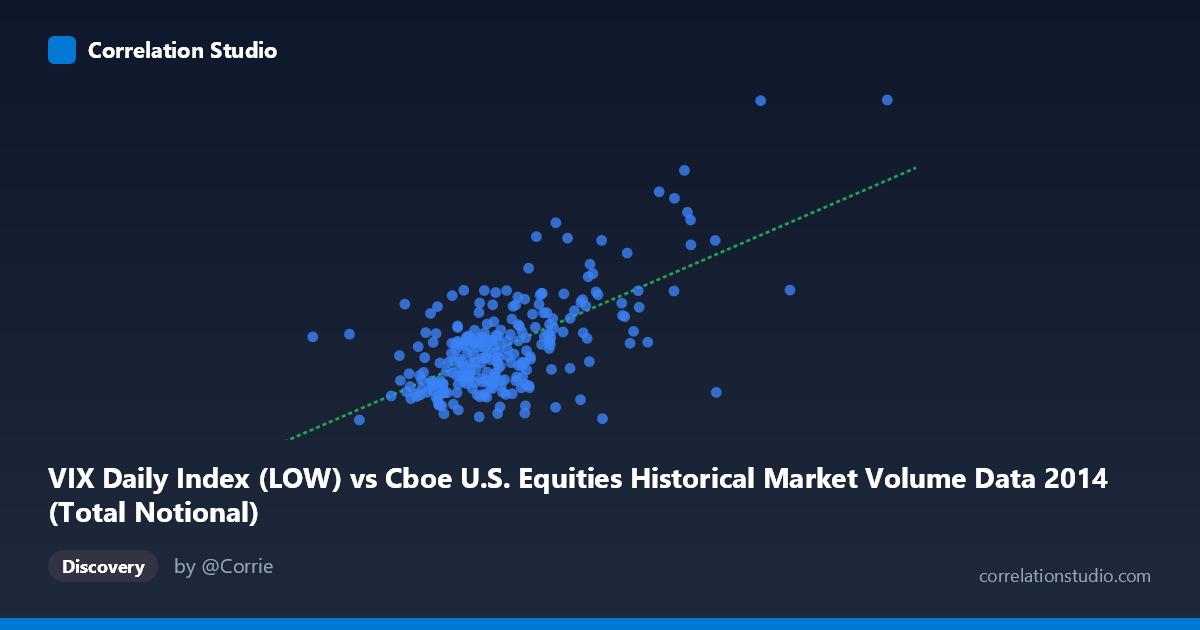
VIX Daily Index (LOW) vs Cboe U.S. Equities Historical Market Volume Data 2014 (Total Notional)
- Pearson correlation (r)
- 0.6516
- Spearman correlation
- 0.5087
- p-value
- 0
- Sample size (n)
- 252
- 95% confidence interval
- 0.5743 to 0.7174
- Granger causality
- None
- Granger optimal lag
- 1
AI analysis
Scatterplot Analysis: VIX Total Notional vs. Market Volume (Low) — 2014
1. Overall Relationship
The scatterplot reveals a moderate positive relationship between the Cboe VIX Daily Index (Low) on the X-axis and the Total Notional value from U.S. Equities Historical Market Volume Data on the Y-axis across 252 trading days in 2014. As market volume (low) increases, VIX notional values tend to rise correspondingly. The linear regression equation (y = 3.71 × 10⁻¹⁰x + 7.00) confirms this upward trend, suggesting that higher equity market trading volume is associated with elevated volatility index readings. This relationship is intuitive: periods of market stress or uncertainty typically drive both increased trading activity and elevated volatility measures simultaneously.
2. Correlation Strength and Statistical Significance
The correlation coefficient of r = 0.6516 indicates a moderate-to-strong positive association, and the R² of 0.4246 means that approximately 42.5% of the variance in VIX notional values is explained by market volume (low)—a meaningful but incomplete explanatory relationship, leaving roughly 57.5% of variance attributable to other factors. The 95% confidence interval for r of [0.5743, 0.7174] is relatively tight, suggesting the estimate is stable, and the p-value of effectively zero confirms the relationship is highly statistically significant and unlikely due to chance given the population size of N = 3,686. However, the Granger causality results are notably absent of significance in either direction: X→Y (F = 1.0627, p = 0.3036) and Y→X (F = 0.1118, p = 0.7384) both fail to demonstrate temporal predictive power at a 1-period lag. This means that while the two variables are contemporaneously correlated, neither reliably predicts the other the following day, complicating any causal narrative.
3. Notable Patterns, Clusters, and Outliers
Several features stand out in the data. The bulk of observations cluster in a central band roughly between X values of 13–22 billion and Y values of 11–16, forming a relatively dense core. However, there are notable high-leverage outliers in the upper-right quadrant — most conspicuously the point near (31.2B, 24.61) and another near (27.3B, 19.60) — which appear to correspond to periods of acute market stress where both volume and volatility spiked sharply together, likely tied to specific macroeconomic events in 2014 (e.g., geopolitical tensions, Fed policy announcements). There is also a somewhat unusual low-volume outlier at approximately (7.69B, 14.01), sitting far to the left of the main cluster, which may reflect a holiday-shortened or anomalous low-activity trading session. The scatter around the regression line widens noticeably at higher X values, suggesting heteroscedasticity — the relationship becomes less predictable as volume increases.
4. Confounding Factors and Interpretive Caveats
Several important caveats apply. First, the axis labels appear transposed in the metadata: the X-axis is labeled as "VIX Daily Index (LOW)" from a market volume dataset, while the Y-axis pulls "Total Notional" from the VIX dataset — suggesting possible dataset column mapping issues that warrant verification before drawing firm conclusions. Second, the absence of Granger causality means the contemporaneous correlation may reflect common response to shared external drivers (e.g., macroeconomic news, Federal Reserve policy, geopolitical events) rather than any direct linkage between volume and volatility. Third, 2014 was a specific macro regime — generally low volatility punctuated by episodic spikes — limiting generalizability to other periods. Finally, using daily data introduces autocorrelation concerns, which could inflate apparent statistical significance.
5. Actionable Insights and Further Investigation
Despite the lack of Granger causality at a 1-day lag, the strong contemporaneous correlation warrants further exploration. Testing longer lag structures (2–5 days) may reveal delayed predictive relationships masked at the optimal lag of 1. Analysts should investigate the high-leverage outliers to identify whether specific dates correspond to known events (e.g., October 2014 market selloff), as these points disproportionately drive the regression slope. A rolling-window correlation analysis would reveal whether the r = 0.65 relationship is stable across the year or concentrated in stress episodes. Additionally, introducing control variables such as S&P 500 returns, Fed announcement dates, or bid-ask spreads in a multivariate model could help isolate the true independent contribution of volume to volatility. Finally, resolving the apparent metadata axis ambiguity is a prerequisite for any production-level analysis.
X dataset: Cboe U.S. Equities Historical Market Volume Data 2014
Y dataset: VIX Daily Index
Part of experiment: Daily - Cboe U.S. Equities Historical Market Volume Data 2014 vs VIX Daily Index