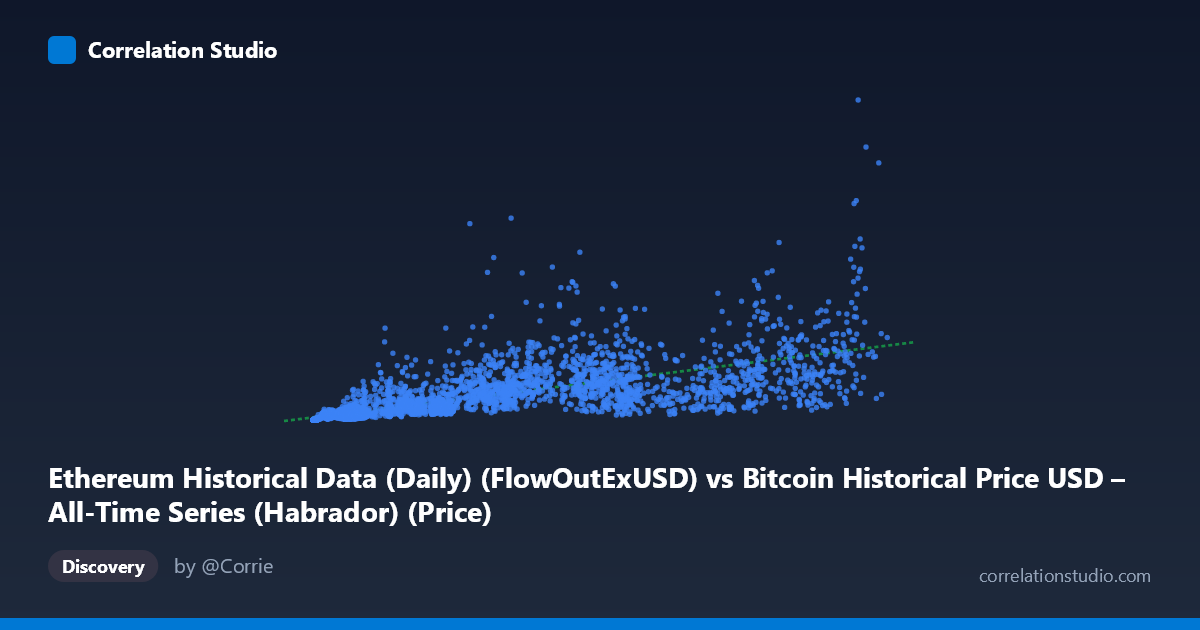
Ethereum Historical Data (Daily) (FlowOutExUSD) vs Bitcoin Historical Price USD – All-Time Series (Habrador) (Price)
- Pearson correlation (r)
- 0.7133
- Spearman correlation
- 0.8996
- p-value
- 0
- Sample size (n)
- 3917
- 95% confidence interval
- 0.6975 to 0.7283
- Granger causality
- None
- Granger optimal lag
- 10
AI analysis
Analysis: Ethereum FlowOutExUSD vs. Bitcoin Price Relationship
1. What the visualization reveals
The scatterplot shows a positive, moderately strong association between Ethereum's exchange flow-out volume (X) and Bitcoin's price (Y). As flow-out values increase, Bitcoin price tends to rise as well, but the relationship is far from a tight linear band — there is substantial vertical spread at every X value, especially in the middle range (X ≈ 10,000–70,000), where Y values scatter across nearly two orders of magnitude (from tens of millions to billions). This spread pattern, combined with the note that Spearman's ρ exceeds Pearson's r, strongly suggests the true relationship is curved (likely logarithmic or power-law) rather than linear — consistent with the fact that both variables span multiple orders of magnitude (X: ~209 to ~124,720; Y: ~13,918 to ~7.36 billion).
2. Strength, direction, and statistical confidence
The Pearson correlation (r = 0.7133) indicates a moderately strong positive linear relationship, but r² = 0.5087 means only about 51% of the variance in Bitcoin price is explained by flow-out volume — leaving nearly half unexplained by this single variable. The 95% CI [0.6975, 0.7283] is narrow, and the p-value of 0 confirms the correlation is highly statistically significant and not due to chance, aided by the large sample size (n = 3,917). However, statistical significance here reflects sample size more than practical predictive power — r² of ~0.51 leaves considerable room for other drivers. Critically, the Granger causality tests (X→Y: p=0.142; Y→X: p=0.229) show no significant temporal predictive direction in either direction at the optimal 10-period lag. This means that despite the contemporaneous correlation, neither variable reliably precedes or forecasts the other in time — the association is likely driven by both series responding to a common underlying factor (e.g., overall crypto market cycles) rather than one causing the other.
3. Notable patterns and outliers
Several notable features emerge: (a) at low X values (<1,000), Y values are uniformly small (thousands to low millions), forming a distinct dense cluster — this likely reflects early historical data (2015–2016) when both Ethereum activity and Bitcoin price were minimal; (b) a fan-shaped spread opens up as X increases, with high-Y outliers appearing across mid-range X values (e.g., X≈20,298 paired with Y≈1.2B, X≈42,772 paired with Y≈1.76B) suggesting periods where Bitcoin price surged independent of proportional flow-out increases (likely 2021 or 2024–2025 bull-run periods); (c) the single most extreme point (X=118,410, Y=7.36B) is a strong high-leverage outlier that could disproportionately influence the linear fit. The heteroscedastic "cone" shape (variance increasing with X) is a classic sign that a log-log transformation would produce a better-fitting, more homoscedastic model.
4. Confounding factors and caveats
The most important caveat is a conceptual mismatch in the axis labels: the dataset descriptions indicate X is described as Ethereum flow-out data while the header says "Bitcoin Historical Price," and Y is labeled Bitcoin price but the dataset description references Ethereum gas/transaction metrics. This suggests possible column mislabeling or merge errors between two different datasets — a critical data-quality issue to resolve before drawing conclusions. Additionally, both series are time-ordered market/network variables that are almost certainly non-stationary (trending with the overall crypto market's multi-year growth), which commonly inflates correlation between unrelated trending series (spurious correlation risk). The lack of Granger causality reinforces that this may be a co-trending relationship (both rising over 2015–2026) rather than a genuine causal or predictive link.
5. Suggested next steps
First, verify and correct data provenance/column labeling before further modeling. Second, refit using a log-log or log-linear model given the multiplicative scaling of both variables — this should substantially improve fit quality and interpretability of elasticity (e.g., % change in Y per % change in X). Third, test for non-stationarity (e.g., ADF test) and consider differencing or working with returns/percentage changes rather than levels to avoid spurious trend-driven correlation. Finally, since Granger tests show no clear lead-lag structure, consider introducing a third variable (e.g., overall market cap, BTC dominance, or macro liquidity indicators) as a potential common driver behind both series' comovement.
X dataset: Bitcoin Historical Price USD – All-Time Series (Habrador)
Y dataset: Ethereum Historical Data (Daily)
Part of experiment: Bitcoin - Bitcoin Historical Price USD – All-Time Series (Habrador) vs Ethereum Historical Data (Daily)