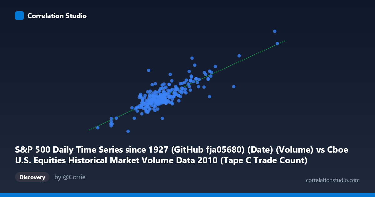
S&P 500 Daily Time Series since 1927 (GitHub fja05680) (Date) (Volume) vs Cboe U.S. Equities Historical Market Volume Data 2010 (Tape C Trade Count)
- Pearson correlation (r)
- 0.8374
- Spearman correlation
- 0.7275
- p-value
- 0
- Sample size (n)
- 252
- 95% confidence interval
- 0.7962 to 0.8709
- Granger causality
- None
- Granger optimal lag
- 10
AI analysis
Analysis: S&P 500 Trading Volume vs. Cboe Tape C Trade Count (2010)
Relationship Overview The scatterplot reveals a strong positive linear relationship between S&P 500 daily trading volume and Cboe Tape C trade count across 252 trading days in 2010. As daily volume increases, the number of discrete trades on Tape C rises proportionally, which is broadly intuitive — higher overall market activity naturally drives more individual transactions. The regression line (y = 6,322.59x + 6.78×10⁸) fits the data reasonably well across the bulk of the distribution, though the relationship shows some heteroscedasticity, with scatter widening at higher volume levels, suggesting the proportionality is not perfectly uniform across the full range.
Correlation Strength and Statistical Significance The Pearson correlation of r = 0.8374 indicates a strong positive association, and the R² of 0.7013 means approximately 70.1% of the variance in Tape C trade counts is explained by aggregate trading volume — a substantial explanatory share for daily financial data. The 95% confidence interval of [0.7962, 0.8709] is notably tight, reflecting the reasonably large sample (n = 252), and the p-value of effectively zero confirms this is not a chance finding. However, the Granger causality results are striking in their absence: neither direction (X→Y: F = 1.13, p = 0.34; Y→X: F = 0.68, p = 0.74) reaches significance at the optimal 10-period lag. This means that while the two variables are strongly contemporaneously correlated, neither reliably predicts the other in a lead-lag temporal sense — they appear to move together rather than one driving the other.
Notable Patterns, Clusters, and Outliers The data exhibits a reasonably tight central cluster between roughly 450,000–750,000 in volume and 3.0–5.5 billion in trade count, representing typical 2010 trading days. Several notable outliers deserve attention: the point near (1,379,287 volume, 9.47 billion trades) sits far to the upper right, likely corresponding to a high-volatility event day. Similarly, the point at (377,050, 1.29 billion) anchors the lower-left extreme. One anomalous point — (1,086,790 volume, 5.45 billion trades) — shows very high volume but a comparatively modest trade count, suggesting a day dominated by large block trades rather than high-frequency small orders, and represents a meaningful deviation from the regression line. These outliers could disproportionately influence the regression slope.
Confounding Factors and Caveats Several important caveats apply. First, Tape C specifically covers NYSE Arca-listed securities, so it captures only a subset of total U.S. equity activity; the correlation reflects a structural relationship between one venue's order fragmentation and aggregate index volume, not necessarily a causal mechanism. Second, both variables are simultaneously driven by common macro factors — volatility events, earnings seasons, Fed announcements, or index rebalancing days — making this largely a case of shared exogenous drivers rather than a direct causal link. Third, 2010 was an unusual year (post-crisis recovery, the May 6 Flash Crash), meaning these patterns may not generalize to other periods. The high-fragmentation trading environment of that era also inflates trade counts independently of economic volume.
Actionable Insights and Further Investigation Practitioners could use this relationship as a real-time proxy signal: if Tape C trade counts deviate significantly from what aggregate volume would predict (i.e., large residuals from the regression), it may signal unusual order fragmentation, algorithmic activity surges, or venue-routing shifts worth investigating. For further analysis, it would be valuable to (1) decompose the outlier days to identify specific market events, (2) test whether the relationship holds in other years to assess structural stability, (3) introduce volatility (VIX) as a control variable to isolate the volume-trade-count relationship from shared volatility drivers, and (4) examine the residuals by time of year to check for seasonality effects such as the year-end liquidity decline visible in some sample points. Extending Granger testing to shorter lags (intraday or 1–3 day) might also reveal finer-grained predictive dynamics not captured at the 10-period optimal lag.
X dataset: Cboe U.S. Equities Historical Market Volume Data 2010
Y dataset: S&P 500 Daily Time Series since 1927 (GitHub fja05680) (Date)
Part of experiment: Daily - Cboe U.S. Equities Historical Market Volume Data 2010 vs S&P 500 Daily Time Series since 1927 (GitHub fja05680) (Date)