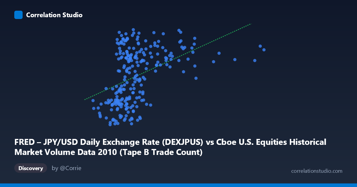
FRED – JPY/USD Daily Exchange Rate (DEXJPUS) vs Cboe U.S. Equities Historical Market Volume Data 2010 (Tape B Trade Count)
- Pearson correlation (r)
- 0.4435
- Spearman correlation
- 0.4681
- p-value
- 0
- Sample size (n)
- 249
- 95% confidence interval
- 0.3378 to 0.5381
- Granger causality
- None
- Granger optimal lag
- 1
AI analysis
Analysis: JPY/USD Exchange Rate vs. Cboe Tape B Trade Count (2010)
Relationship Overview The scatterplot reveals a modest positive relationship between the JPY/USD daily exchange rate (X-axis, representing U.S. equity market volume in notional terms) and the Cboe Tape B Trade Count (Y-axis, representing the yen-per-dollar exchange rate). As the market volume metric increases, trade counts tend to rise gradually, following the linear regression equation y = 1.417×10⁻⁵x + 83.43. However, the relationship is far from clean — substantial vertical scatter is visible across virtually all X-values, indicating that many other forces are at work beyond this single predictor. The data spans the full 2010 calendar year (January through December), capturing a coherent annual market cycle.
Correlation Strength and Statistical Significance The Pearson correlation of r = 0.4435 indicates a moderate positive association, but the explanatory power is limited: R² = 0.1967, meaning only about 19.7% of the variance in Tape B Trade Count is explained by the exchange rate variable. The remaining ~80% of variation is attributable to other factors entirely. The 95% confidence interval of [0.338, 0.538] is meaningfully above zero and reasonably tight, providing reliable evidence that the true population correlation is positive and non-trivial. The p-value of 2.025×10⁻¹³ confirms the result is highly statistically significant given the large population (N = 3,302), essentially ruling out chance as an explanation. Critically, however, the Granger causality tests find no significant predictive directionality in either direction — neither X→Y (F = 0.47, p = 0.495) nor Y→X (F = 0.47, p = 0.494) reaches significance at any conventional threshold. This means that despite the correlation, knowing today's exchange rate does not improve predictions of tomorrow's trade count, and vice versa.
Patterns, Clusters, and Outliers Several structural features stand out in the scatter. The bulk of observations cluster in the X range of roughly 150,000–400,000, with Y values spanning the full range (~81–94), suggesting high variability in trade counts even at typical volume levels. There is a visually apparent right-tail extension — a handful of points with X values exceeding 500,000–900,000 — that likely exerts disproportionate influence on the regression slope and correlation coefficient. These high-volume outliers (e.g., ~676,000 and ~918,000) appear to anchor the upper-right portion of the fit. Additionally, there is a noticeable bifurcated spread at moderate X values: some observations cluster near Y ≈ 83–85 while others at similar X values reach Y ≈ 92–94, hinting at possible regime changes, seasonal effects, or sub-population structure within the 2010 data. No strong non-linear curvature is apparent, but the linear model's modest R² suggests a linear fit may be inadequate.
Confounding Factors and Caveats A critical interpretive caveat is that this correlation likely reflects shared temporal trends rather than direct causation. Both U.S. equity trading volumes and the JPY/USD exchange rate are driven by macro-financial conditions — risk appetite, Federal Reserve policy, global economic uncertainty, and market volatility regimes (e.g., the European sovereign debt crisis in 2010). These common drivers could generate co-movement without any direct mechanical link between the two variables. The column-to-dataset mismatch in the metadata (each variable is attributed to the other's dataset) also warrants careful verification of data integrity before drawing firm conclusions. Furthermore, the large N (3,302) relative to the sample (249) means statistical significance is easily achieved even for economically trivial correlations, making practical significance the more relevant benchmark here.
Actionable Insights and Further Investigation Given that ~80% of variance remains unexplained and Granger causality is absent, practitioners should avoid using the JPY/USD rate as a standalone predictor of Tape B trade counts or vice versa for operational or trading decisions. Further investigation should include: (1) controlling for VIX or realized volatility to test whether shared volatility regimes explain the correlation; (2) segmenting by month or quarter to determine if the relationship is stronger in specific periods (e.g., the yen carry-trade dynamics of mid-2010); (3) testing non-linear specifications or threshold models that might better capture the bifurcated distribution observed at moderate X values; and (4) expanding to multi-year data to test whether the 2010 correlation is stable or an artifact of that particular macro environment. A multivariate framework incorporating volume from other tapes, broader currency baskets, and volatility indices would likely yield substantially more explanatory power.
X dataset: Cboe U.S. Equities Historical Market Volume Data 2010
Y dataset: FRED – JPY/USD Daily Exchange Rate
Part of experiment: Daily - Cboe U.S. Equities Historical Market Volume Data 2010 vs FRED – JPY/USD Daily Exchange Rate