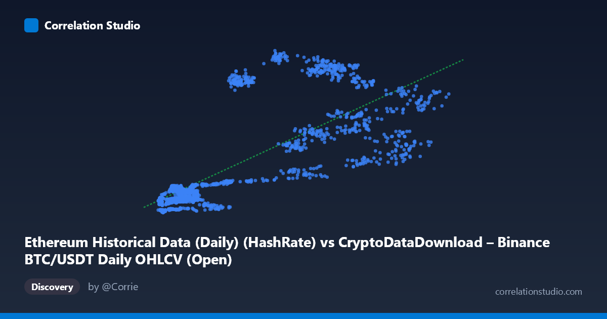
Ethereum Historical Data (Daily) (HashRate) vs CryptoDataDownload – Binance BTC/USDT Daily OHLCV (Open)
- Pearson correlation (r)
- 0.7515
- Spearman correlation
- 0.7567
- p-value
- 0
- Sample size (n)
- 1855
- 95% confidence interval
- 0.731 to 0.7706
- Granger causality
- None
- Granger optimal lag
- 1
- Time coverage
- 2017-08-17 to 2022-09-14
AI analysis
Analysis: Ethereum Hash Rate vs. Binance BTC/USDT Opening Price
1. What the Visualization Reveals
The scatterplot shows a positive, moderately strong monotonic relationship between the X variable (labeled here as Ethereum Hash Rate, though the axis metadata is inconsistent with the data description) and Y (BTC/USDT opening price). As X increases from the low thousands to the mid-tens-of-thousands range, Y rises from roughly 100–200 up to 800–1000+. However, the spread of points widens considerably at higher X values, suggesting the relationship is not perfectly linear and that variance in Y grows with X (heteroscedasticity).
2. Strength, Direction, and Uncertainty
The correlation coefficient (r = 0.75) indicates a fairly strong positive linear relationship, with r² = 0.565 meaning only about 56% of the variance in Y is explained by X — leaving nearly 44% attributable to other factors, noise, or nonlinear dynamics not captured by this simple linear model. The 95% confidence interval [0.731, 0.771] is tight, and the p-value ≈ 0 confirms this correlation is highly statistically significant and not due to chance, largely a function of the large sample size (n=1,855). However, statistical significance here should not be conflated with predictive or causal strength — r² makes clear that substantial unexplained variance remains.
Critically, the Granger causality tests show no significant predictive direction in either direction (X→Y: p=0.264; Y→X: p=0.474). This means that past values of one variable do not meaningfully help forecast future values of the other at a 1-period lag. This is an important caveat: despite the strong contemporaneous correlation, there is no evidence of temporal lead-lag structure — the two series likely move together due to a shared underlying driver (e.g., overall crypto market sentiment, capital inflows, or time trend) rather than one causing the other.
3. Notable Patterns and Outliers
Several clusters are visible: - A dense cluster of points at low X (3,000–12,000) with Y mostly between 100–250, showing tight, low-variance behavior. - A sparser but highly variable cluster at higher X (20,000–55,000) where Y ranges dramatically from ~270 to over 1000 for similar X values (e.g., X≈53,785 gives Y=715, while X≈29,445 gives Y=1016). This suggests a regime change or the influence of a third factor (like time/date) once X exceeds ~20,000. - Notable outliers include (20,468.81, 939.71) and (21,310.90, 873.68) — high Y values at relatively moderate X, breaking the general trend and pulling toward nonlinearity.
This pattern is consistent with two possible regimes: a "low-activity" phase with compressed values and a "high-activity/bull market" phase with amplified, more volatile values.
4. Confounding Factors and Caveats
- Time confound: Both hash rate and price often trend upward over multi-year periods due to overall market growth/adoption. Since data spans 2017–2022, both series may simply share a common time trend rather than a direct functional relationship — classic spurious correlation risk with non-stationary time series. - Metadata mismatch: The column descriptions are contradictory (X labeled "Hash Rate" from a BTC dataset, Y labeled BTC OHLCV Open from an Ethereum dataset) — this suggests possible data-labeling errors that should be verified before drawing conclusions. - Non-stationarity: Crypto price/hash rate series are typically non-stationary (trending, autocorrelated), which can inflate correlation estimates and invalidate standard significance tests unless differenced or detrended first. - Heteroscedasticity: Variance in Y increases with X, violating linear regression assumptions and reducing reliability of the fitted line at higher ranges.
5. Recommendations for Further Investigation
- Verify data labels/sources — resolve the inconsistency between axis descriptions before further analysis. - Detrend or difference both series (e.g., use % daily returns instead of levels) and re-test correlation/Granger causality on stationary series to rule out spurious trend-driven correlation. - Segment analysis by time period or regime (e.g., pre/post 2021 bull run) to check whether the relationship is stable or driven by a specific market phase. - Explore nonlinear or lagged models (e.g., polynomial fits, VAR with additional lags, or machine learning regressors) given the fan-shaped variance pattern and lack of simple lag-1 Granger causality. - Investigate a third common factor (e.g., overall market cap, BTC price, network adoption metrics) that may drive both variables simultaneously, explaining the correlation without direct causality.
X dataset: CryptoDataDownload – Binance BTC/USDT Daily OHLCV
Y dataset: Ethereum Historical Data (Daily)
Part of experiment: Bitcoin - CryptoDataDownload – Binance BTC/USDT Daily OHLCV vs Ethereum Historical Data (Daily)