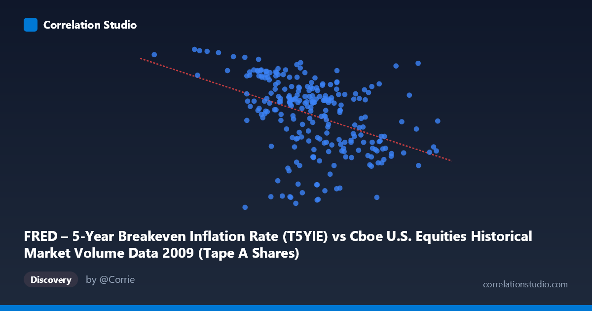
FRED – 5-Year Breakeven Inflation Rate (T5YIE) vs Cboe U.S. Equities Historical Market Volume Data 2009 (Tape A Shares)
- Pearson correlation (r)
- -0.422
- Spearman correlation
- -0.4573
- p-value
- 0
- Sample size (n)
- 250
- 95% confidence interval
- -0.5189 to -0.3144
- Granger causality
- None
- Granger optimal lag
- 1
AI analysis
Scatterplot Analysis: 5-Year Breakeven Inflation Rate vs. Cboe U.S. Equities Market Volume (2009)
Relationship Overview
The scatterplot reveals a moderate negative relationship between U.S. equity market trading volume (X-axis) and the 5-Year Breakeven Inflation Rate (Y-axis) across the 2009 trading year. As daily equity volume increases, inflation expectations as measured by the TIPS-derived breakeven rate tend to decline. The linear regression equation (y = -2.348E-09x + 2.172) confirms this inverse slope, meaning that for every ~426 million additional shares traded, the breakeven inflation rate decreases by roughly one percentage point. Visually, the data points form a downward-sloping cloud, with higher breakeven rates (above 1.5%) concentrated at lower volume levels and lower breakeven readings (below 0.75%) appearing more frequently at higher volume levels — though considerable scatter surrounds this trend throughout.
Correlation Strength and Statistical Significance
The Pearson correlation of r = -0.422 indicates a moderate negative association, and the r² of 0.178 means that approximately 17.8% of the variance in inflation expectations is statistically explained by equity trading volume. While this is non-trivial, it also means that roughly 82% of the variation remains unexplained by this linear relationship alone. The 95% confidence interval of [-0.519, -0.314] is entirely negative and does not cross zero, reinforcing directional confidence, and the p-value of 3.2E-12 confirms the relationship is highly statistically significant — essentially ruling out chance given the sample of 250 paired observations drawn from a population of 3,232. However, the Granger causality tests tell a critically different story: neither variable temporally predicts the other (X→Y: F=0.000, p=0.998; Y→X: F=0.325, p=0.569). This means the correlation, while real in a cross-sectional sense, carries no evidence of temporal predictive power — knowing yesterday's volume does not help forecast today's inflation expectations, and vice versa.
Notable Patterns, Clusters, and Outliers
Several features stand out in the data. A cluster of points with high breakeven rates (1.8–2.13) appears predominantly at lower volume ranges (roughly 105M–350M), which likely corresponds to the recovery period later in 2009 as markets stabilized and inflation expectations rebounded from crisis lows. Conversely, points at the highest volume levels (600M–704M) tend to cluster at very low breakeven rates (0.3–0.7), consistent with early 2009 when extreme market stress drove both panic-driven volume surges and near-deflationary expectations. A few notable outliers are visible: the point at approximately (376M, -0.08) represents a rare negative breakeven reading — implying brief market pricing of deflation — and (105M, 2.05) sits at an extreme low-volume, high-inflation-expectation position. The data also shows heteroscedasticity, with variance in breakeven rates appearing widest at mid-range volume levels and compressing at the extremes.
Confounding Factors and Interpretive Caveats
The 2009 timeframe is a critical caveat. This was an extraordinarily unusual year dominated by the aftermath of the 2008 financial crisis, the market bottom in March 2009, and the subsequent recovery — a regime with few historical parallels. Both variables were likely jointly driven by a common third factor: systemic financial stress and risk sentiment. During peak fear, volume surged (panic selling, forced deleveraging) while inflation expectations collapsed toward deflation; as fear receded, volume normalized and inflation expectations recovered. This shared dependence on a latent risk/fear factor likely explains much of the observed correlation without implying any direct causal mechanism between volume and inflation pricing. Additionally, the axes appear to be swapped from conventional labeling (the dataset descriptions suggest X is volume and Y is the inflation rate, but the source notes indicate the axis labels may be reversed), which warrants verification before drawing firm conclusions. Survivorship bias in which trading days are included and the use of daily rather than intraday data also limit interpretive precision.
Actionable Insights and Further Investigation
Given the lack of Granger causality, practitioners should not attempt to use equity volume as a leading indicator for inflation breakeven rates or vice versa for trading or forecasting purposes. However, the moderate contemporaneous correlation does suggest both series respond to common macro drivers worth isolating. Recommended next steps include: (1) incorporating a volatility index (e.g., VIX) or credit spreads as a control variable to test whether the volume–inflation correlation disappears once risk sentiment is held constant; (2) extending the analysis beyond 2009 to assess whether this relationship persists across different market regimes or is purely crisis-specific; (3) applying rolling-window correlation analysis to identify whether the relationship strengthens or weakens at particular phases of the business cycle; and (4) testing non-linear models (e.g., polynomial or regime-switching), given the visible clustering at the extremes that a single linear fit may inadequately capture. The 17.8% explained variance, while modest, is large enough to motivate deeper structural modeling rather than dismissal.
X dataset: Cboe U.S. Equities Historical Market Volume Data 2009
Y dataset: FRED – 5-Year Breakeven Inflation Rate
Part of experiment: Daily - Cboe U.S. Equities Historical Market Volume Data 2009 vs FRED – 5-Year Breakeven Inflation Rate