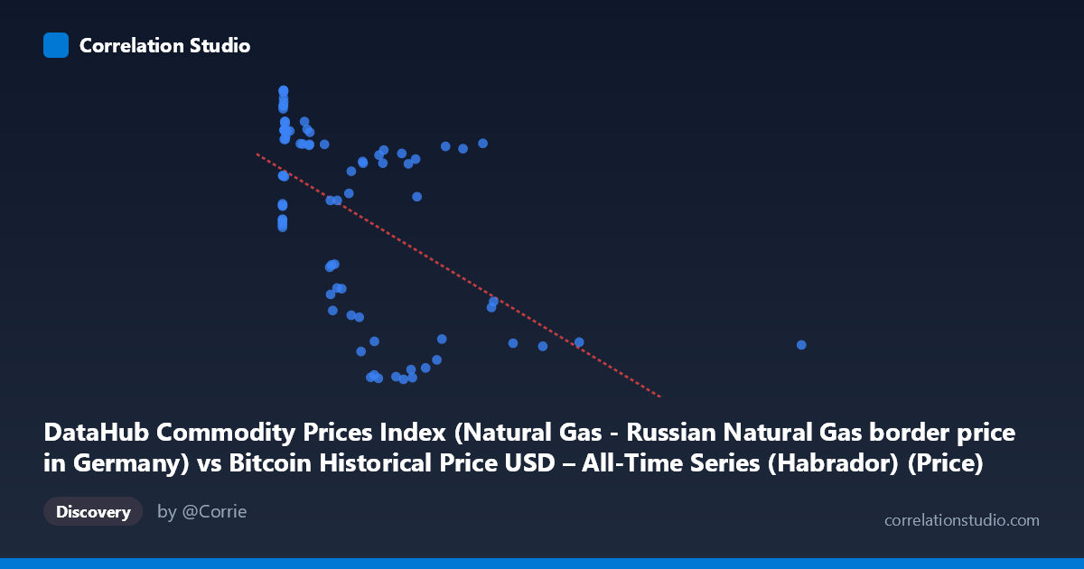
DataHub Commodity Prices Index (Natural Gas - Russian Natural Gas border price in Germany) vs Bitcoin Historical Price USD – All-Time Series (Habrador) (Price)
- Pearson correlation (r)
- -0.5559
- Spearman correlation
- -0.5373
- p-value
- 0
- Sample size (n)
- 83
- 95% confidence interval
- -0.689 to -0.3866
- Granger causality
- None
- Granger optimal lag
- 1
AI analysis
Analysis of Natural Gas Price Index vs. Bitcoin Price Relationship
1. Visual Relationship Overview
The scatterplot shows a downward-sloping, non-linear pattern between the Russian natural gas border price index (X) and Bitcoin's historical price (Y). Rather than a clean linear trend, the data reveals a distinctive pattern: at low X-values (roughly 0–100), Y-values are widely scattered across nearly the full range (8.5–12.6), while at higher X-values (400), Y-values cluster into two bands — one low (~4–6) and one high (~9.5–11). This bifurcation suggests the relationship is not a simple continuous decay but may reflect distinct time regimes or market phases.
2. Correlation Strength and Statistical Confidence
The correlation coefficient (r = -0.556, r² = 0.309) indicates a moderate negative relationship, with only 30.9% of the variance in Y explained by X — meaning roughly 70% of Bitcoin price movement is driven by other factors entirely. The 95% CI [-0.689, -0.387] is reasonably tight and excludes zero, and the p-value (4.87e-08) confirms this correlation is statistically significant and unlikely due to chance. However, statistical significance here reflects a real but weak-to-moderate association, not a strong predictive relationship. Critically, the Granger causality tests show no significant predictive direction in either direction (X→Y: p=0.18; Y→X: p=0.08, only marginally suggestive). This means neither variable reliably "leads" the other in time — the correlation is likely coincidental co-trending rather than a causal or predictive relationship.
3. Notable Patterns and Outliers
Several structural features stand out: - Low-X cluster (X < 20): A tight vertical band near X≈0–20 with Y ranging from 8.5 to 12.6 — likely representing Bitcoin's early history (2010-2013) when prices were near-zero and gas prices were also low. - Bimodal split at high X: For X 400, Y values split into two clear groups (~4-5 and ~10-11), suggesting different time periods with similar gas prices but very different Bitcoin valuations — a hallmark of a time-series artifact rather than genuine covariation. - Extreme X outlier: The point (2452.18, 4.98) is far outside the typical X range and could be exerting outsized leverage on the regression slope.
4. Confounding Factors and Caveats
This is a classic case of spurious correlation via shared time trends. Both series span 2010–2017 and are independently trending (Bitcoin through adoption cycles, gas prices through global energy markets), making any correlation a byproduct of trending time-series data rather than an economic relationship. Neither variable has an obvious causal mechanism linking Russian gas border prices to Bitcoin valuations. The non-significant Granger results reinforce this: true causal or leading relationships would show predictive power in at least one direction. Additionally, unequal time-sampling and potential autocorrelation within each series (not accounted for by simple Pearson r) can inflate apparent correlation strength.
5. Recommendations for Further Investigation
Given the weak explanatory power and lack of Granger causality, this pairing should be treated as non-causal and likely spurious for forecasting purposes. To validate or refute this, analysts should: (1) detrend both series (e.g., first-difference or log-return transforms) and re-test correlation to see if it disappears — a common result for trending, unrelated series; (2) test against a macro confound like global risk sentiment, USD strength, or overall commodity indices, which may better explain co-movement in both; and (3) avoid using natural gas prices as a Bitcoin price predictor in any trading or economic model given the absence of temporal lead-lag structure.
X dataset: Bitcoin Historical Price USD – All-Time Series (Habrador)
Y dataset: DataHub Commodity Prices Index
Part of experiment: Bitcoin - Bitcoin Historical Price USD – All-Time Series (Habrador) vs DataHub Commodity Prices Index