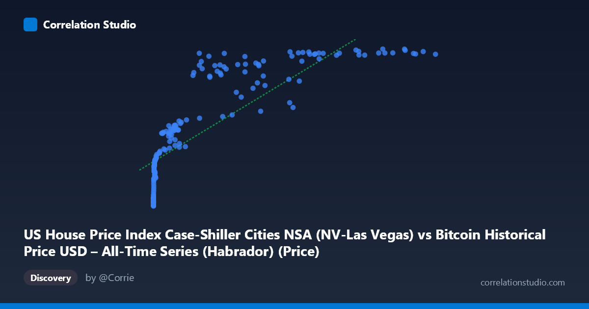
US House Price Index Case-Shiller Cities NSA (NV-Las Vegas) vs Bitcoin Historical Price USD – All-Time Series (Habrador) (Price)
- Pearson correlation (r)
- 0.8155
- Spearman correlation
- 0.9662
- p-value
- 0
- Sample size (n)
- 187
- 95% confidence interval
- 0.761 to 0.8585
- Granger causality
- None
- Granger optimal lag
- 9
AI analysis
Analysis: Bitcoin Price vs. Las Vegas Case-Shiller Home Price Index
1. What the Visualization Reveals
The scatterplot shows a strong positive association between Bitcoin's price (X-axis, note the axis labels appear swapped based on the data description) and the Las Vegas Case-Shiller housing index. At low Bitcoin prices (under $1,000), the housing index clusters tightly between ~90-160. As Bitcoin prices climb into the tens of thousands, the housing index rises correspondingly into the 250-306 range. The relationship is not a clean straight line — it has a pronounced curved, compressive shape: rapid index growth at low X values, followed by a flattening/plateau effect as X grows very large (index values ceiling near 300-306 even as X ranges from 60,000 to 118,670).
2. Strength, Direction, and Statistical Meaning
The Pearson correlation (r = 0.8155, r² = 0.665) indicates a strong positive linear relationship, with about 66.5% of the variance in the housing index statistically explained by Bitcoin price levels. The 95% CI [0.761, 0.859] is tight and excludes zero, and the p-value of ~0 confirms this correlation is highly unlikely due to chance. However, the note that Spearman ρ exceeds Pearson r is important — it signals the true relationship is monotonic but non-linear, meaning a log or power-curve fit would likely explain notably more variance than the reported 66.5% linear R². Critically, the Granger causality tests (p = 0.72 and p = 0.78, both non-significant) show no evidence of temporal predictive power in either direction. This means despite the strong contemporaneous correlation, neither series' past values help forecast the other's future values — the correlation is coincidental co-movement, not a lead-lag causal signal.
3. Notable Patterns and Features
- Curvature/saturation: The clearest non-linear feature is the ceiling effect above X≈50,000, where housing index values compress into a narrow 280-306 band despite X more than doubling. This is classic logarithmic/diminishing-returns behavior. - Low-end clustering: Points with X < 20 (e.g., 0.06, 0.20, 3-15) form a dense cluster with Y between 89-105, essentially a floor. - Mid-range scatter: Between X = 20,000-60,000, there's more vertical spread (e.g., 45,092→220 vs. 44,354→283), suggesting other factors or timing noise affect the relationship in this zone. - No obvious outliers — the data follows a consistent monotonic envelope, just not a straight one.
4. Confounding Factors and Caveats
This is almost certainly a spurious correlation driven by shared time trends, not a causal economic relationship. Both series have risen substantially over the 2010-2026 window covered by the data — Bitcoin due to adoption/speculation cycles, and Las Vegas housing due to broader US real estate appreciation, low interest rates (2010s), post-COVID housing booms, and migration trends. Any two upward-trending time series over the same period will show inflated correlation from shared temporal drift, independent of true linkage. Additionally, mismatched sampling (n=187 paired vs. population 470) and NSA (non-seasonally-adjusted) housing data introduce potential aggregation and alignment noise. The lack of Granger causality strongly supports the "spurious trend correlation" interpretation over any genuine predictive/causal mechanism.
5. Actionable Insights & Further Investigation
- Re-fit with a log-transform: Given the Spearman/Pearson divergence and visible saturation curve, try y = a·ln(x) + b or a power/logistic model — this should meaningfully improve R² beyond 66.5%. - De-trend both series (e.g., using year-over-year % changes or differencing) and re-test correlation and Granger causality on the detrended/stationary series to check if the relationship survives — this is the standard fix for spurious time-trend correlation. - Avoid causal claims or trading/investment strategies based on this correlation given the null Granger result; treat it as coincidental macro co-trending (both assets benefited from the same low-rate, high-liquidity macro environment post-2010). - Segment by market regime (e.g., pre-2017 vs. 2017-2021 vs. post-2022) to see if the relationship strength or shape changes across Bitcoin's distinct bull/bear cycles, which may reveal it's an artifact of a few shared macro periods rather than a stable structural relationship.
X dataset: Bitcoin Historical Price USD – All-Time Series (Habrador)
Y dataset: US House Price Index Case-Shiller Cities NSA
Part of experiment: Bitcoin - Bitcoin Historical Price USD – All-Time Series (Habrador) vs US House Price Index Case-Shiller Cities NSA