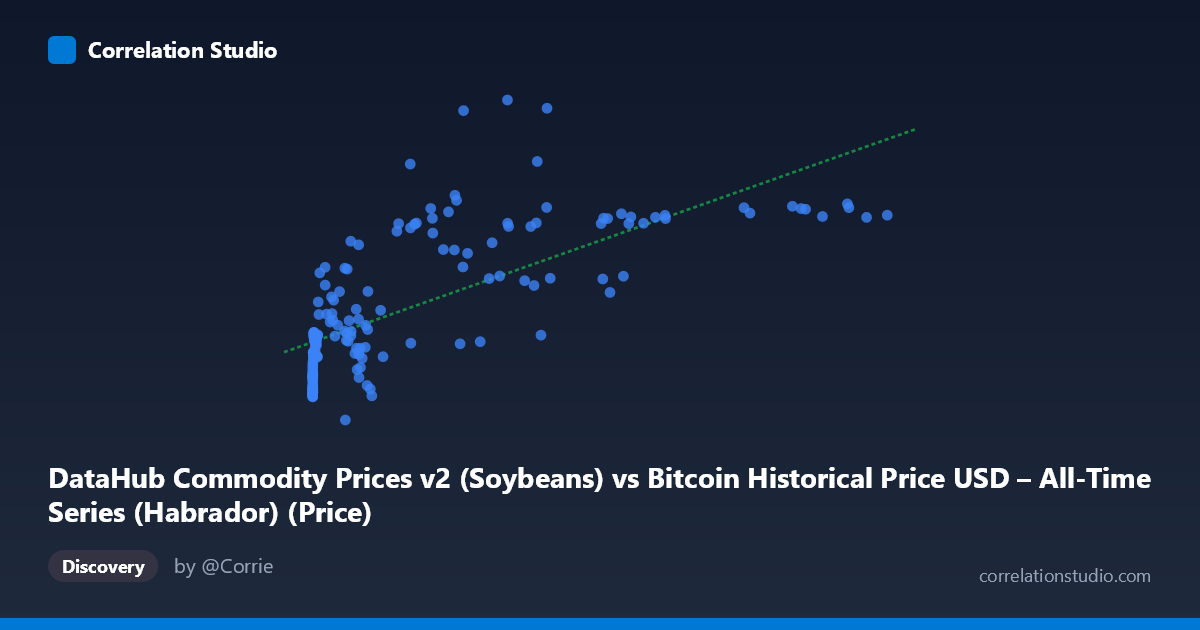
DataHub Commodity Prices v2 (Soybeans) vs Bitcoin Historical Price USD – All-Time Series (Habrador) (Price)
- Pearson correlation (r)
- 0.7187
- Spearman correlation
- 0.8084
- p-value
- 0
- Sample size (n)
- 182
- 95% confidence interval
- 0.6402 to 0.7824
- Granger causality
- None
- Granger optimal lag
- 1
AI analysis
Analysis: Bitcoin Price vs. Soybean Prices
1. What the Visualization Reveals
The scatterplot shows a positive but noticeably non-linear relationship between Bitcoin's historical USD price (X-axis) and soybean commodity prices (Y-axis). Given the massive range of Bitcoin values (from $0.06 to $113,500), the data is heavily right-skewed, with most points clustered at low X-values (under $50,000) and a long tail extending to Bitcoin's all-time highs. Soybean prices, by contrast, occupy a much narrower and more stable range ($73.86–$227.96). The pattern resembles a logarithmic or saturating curve more than a straight line—soybean prices rise steeply as Bitcoin moves from near-zero to the thousands, then the relationship flattens and becomes noisier at higher Bitcoin valuations.
2. Strength, Direction, and Statistical Confidence
The Pearson correlation of r = 0.719 indicates a moderately strong positive linear association, with r² = 0.517 meaning Bitcoin's price statistically explains about 52% of the variance in soybean prices—leaving nearly half unexplained by this simple linear model. The 95% confidence interval [0.640, 0.782] is reasonably tight and excludes zero, and the p-value (~0) confirms this correlation is highly unlikely to be due to chance, especially given n=182. However, statistical significance here should not be confused with causal or economically meaningful linkage. Critically, the Granger causality tests show no significant predictive direction in either direction (X→Y: p=0.869; Y→X: p=0.664). This strongly suggests the correlation is not driven by one variable temporally leading the other—rather, both series likely trend upward together over the 2010–2025 window due to shared macro conditions (e.g., inflation, dollar weakness, broad asset appreciation) rather than any direct market interaction.
3. Notable Patterns and Outliers
Several features stand out: - Early-era clustering: Many low-X points (Bitcoin under $50) correspond to soybean prices in the 86–100 range, forming a tight cluster that anchors the low end of the curve. - Curvature: The relationship flattens/plateaus in the 20,000–50,000 range, with visible scatter—e.g., (33087, 111.57) and (10741, 90.48) are low-soybean-price outliers relative to their high Bitcoin values, breaking the expected upward trend. - High-value volatility: At the top of the Bitcoin range (X 40,000), Y-values vary widely (111.57 to 227.96), indicating the relationship weakens or becomes noisy precisely where Bitcoin experienced its most extreme price action (bull runs/crashes). - Possible bimodality: The concentration of points at very low X-values combined with a sparse but wide-ranging upper tail suggests the linear model is overly simplistic for this data structure.
4. Confounding Factors and Caveats
This correlation is almost certainly spurious or indirect, driven by shared temporal trends rather than direct economic linkage: - Time-trend confounding: Both Bitcoin adoption/price growth and long-term commodity inflation have risen over the 2010–2025 period. Two unrelated series that both trend upward over time will show spurious correlation. - Non-stationarity: Neither series is likely stationary (both have long-term drift), which inflates correlation estimates and can produce misleading regression fits—a classic time-series pitfall. - Scale mismatch: Bitcoin's range spans 6 orders of magnitude while soybeans span roughly 3-fold—this heteroscedasticity means the linear R² is disproportionately influenced by extreme X-values. - No mechanistic link: There's no obvious economic mechanism connecting soybean futures pricing to Bitcoin valuation; both are more plausibly responding to macro liquidity, inflation expectations, or USD strength independently.
5. Actionable Insights and Further Investigation
Given the lack of Granger causality, this correlation should not be used for predictive trading or hedging strategies between these two assets. Instead: - Detrend both series (e.g., using log-returns or first differences) and re-test correlation—this will likely reveal whether any genuine short-term co-movement exists once the shared upward trend is removed. - Introduce a common macro variable (e.g., CPI, DXY dollar index, M2 money supply) as a control to test whether both series are simply proxying for the same underlying driver. - Log-transform Bitcoin's X-axis given its extreme skew—this would likely improve model fit and reveal whether the true relationship is logarithmic rather than linear. - Treat the current r²=0.517 as descriptive, not causal or predictive—it quantifies co-trending, not a tradeable or economically actionable relationship.
X dataset: Bitcoin Historical Price USD – All-Time Series (Habrador)
Y dataset: DataHub Commodity Prices v2
Part of experiment: Bitcoin - Bitcoin Historical Price USD – All-Time Series (Habrador) vs DataHub Commodity Prices v2