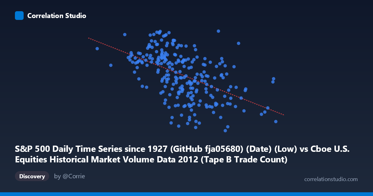
S&P 500 Daily Time Series since 1927 (GitHub fja05680) (Date) (Low) vs Cboe U.S. Equities Historical Market Volume Data 2012 (Tape B Trade Count)
- Pearson correlation (r)
- -0.5083
- Spearman correlation
- -0.5572
- p-value
- 0
- Sample size (n)
- 250
- 95% confidence interval
- -0.5949 to -0.4101
- Granger causality
- X → Y
- Granger optimal lag
- 1
AI analysis
Analysis: S&P 500 Daily Low vs. Cboe Tape B Trade Count (2012)
Relationship Overview The scatterplot reveals a moderate negative relationship between the S&P 500 daily low price (X) and the Cboe Tape B trade count (Y) across 2012. As the S&P 500's daily low price increases — reflecting generally rising equity valuations throughout the year — the number of Tape B trades tends to decrease. The linear regression equation (y = −0.00061x + 1,477.62) captures this downward trend, suggesting that higher index levels correspond with fewer discrete trades on Cboe's Tape B venues. This is a somewhat counterintuitive pattern at first glance, but it reflects a well-documented phenomenon in equity market microstructure: rising markets are often accompanied by declining trading frequency as uncertainty and urgency to transact diminish.
Correlation Strength and Statistical Significance The Pearson correlation of r = −0.508 indicates a moderate negative association, and the R² of 0.258 means that roughly 25.8% of the variance in Tape B trade counts is explained by the S&P 500 daily low. While statistically meaningful, this also means that nearly 74% of the variance remains unexplained by this single variable alone, underscoring the complexity of trade count dynamics. The 95% confidence interval of [−0.595, −0.410] is entirely negative and relatively tight, providing strong evidence that the true population correlation is genuinely negative and not a sampling artifact. The p-value of ~0 confirms this result is highly statistically significant across the n = 250 paired sample drawn from N = 3,750 observations. Critically, the Granger causality analysis identifies a unidirectional relationship: X Granger-causes Y (F = 5.11, p = 0.025) at a 1-period lag, while Y does not Granger-cause X (F = 0.82, p = 0.365). This means that yesterday's S&P 500 low has measurable predictive power over today's Tape B trade count, but not vice versa — lending a temporal, directional dimension to the correlation that goes beyond mere co-movement.
Patterns, Clusters, and Outliers The scatterplot shows considerable vertical dispersion throughout the X range, consistent with the moderate (rather than strong) correlation. Several notable features emerge from the sample points. There is a visible cluster of high trade counts (Y ≈ 1,390–1,460) concentrated in the lower X range (roughly 100,000–160,000), corresponding to periods when the S&P 500 was trading at lower levels — likely early 2012 or periods of market stress. Conversely, higher X values (200,000+) tend to cluster at lower trade counts (Y ≈ 1,270–1,370). A potential outlier stands out at approximately (222,650; 1,460) — an unusually high trade count despite a relatively elevated index level — which may reflect a specific volatility event or index rebalancing day. The point at (170,460; 1,268) also appears anomalously low in trade count relative to its index level. The spread does not appear to narrow or widen systematically across the X range, suggesting reasonably homoscedastic residuals, though the non-linear curvature cannot be fully ruled out given the scatter.
Confounding Factors and Caveats Several important caveats temper a causal interpretation. First, this is a time-series correlation across a single calendar year (2012), meaning both variables are likely trending — the S&P 500 broadly rose through 2012 while trading volumes were in a secular decline post-2009. This shared temporal trend (spurious co-trending) could be inflating the observed correlation. Second, Tape B specifically covers NYSE American (AMEX) and regional exchange securities, not the full market, so it may not respond identically to broad S&P 500 movements. Third, macroeconomic events, earnings seasons, options expiration cycles, and regulatory changes (e.g., SEC rule changes in 2012) could simultaneously affect both variables without one causing the other. Fourth, while Granger causality suggests predictive directionality, it does not establish structural or economic causation — it is a statistical test sensitive to lag specification and model assumptions. The optimal lag of just 1 period is plausible given daily data but should be validated across multiple lag windows.
Actionable Insights and Further Investigation Practitioners and researchers should consider several follow-up steps. Detrending both series (e.g., via first-differencing or regressing out a common time trend) would help isolate whether the correlation persists beyond shared secular movement. Extending the analysis across multiple years (e.g., 2008–2023) would reveal whether this negative relationship is structurally stable or specific to the low-volatility, rising-market conditions of 2012. Investigating nonlinear specifications (e.g., polynomial regression or spline models) could improve on the 25.8% R² and better capture threshold effects during market stress periods. The Granger causality finding — that the S&P 500 low predicts next-day Tape B trade counts — warrants exploration as a short-term volume forecasting signal, potentially useful for algorithmic execution strategies on Tape B venues. Finally, incorporating additional predictors such as the VIX, intraday volatility, or market breadth indicators into a multivariate model would likely substantially improve explanatory power beyond the 26% captured here.
X dataset: Cboe U.S. Equities Historical Market Volume Data 2012
Y dataset: S&P 500 Daily Time Series since 1927 (GitHub fja05680) (Date)
Part of experiment: Daily - Cboe U.S. Equities Historical Market Volume Data 2012 vs S&P 500 Daily Time Series since 1927 (GitHub fja05680) (Date)