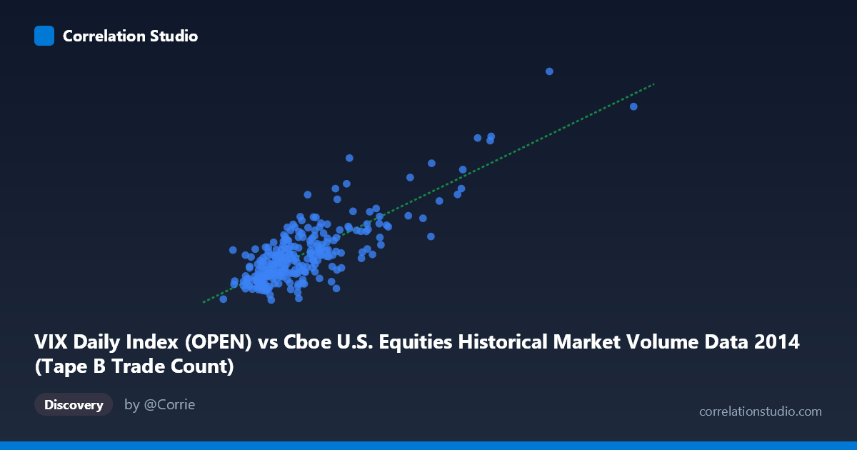
VIX Daily Index (OPEN) vs Cboe U.S. Equities Historical Market Volume Data 2014 (Tape B Trade Count)
- Pearson correlation (r)
- 0.8124
- Spearman correlation
- 0.6878
- p-value
- 0
- Sample size (n)
- 252
- 95% confidence interval
- 0.7657 to 0.8506
- Granger causality
- None
- Granger optimal lag
- 1
AI analysis
Scatterplot Analysis: VIX Open vs. Tape B Trade Count (2014)
Overview of the Relationship
The scatterplot reveals a clear positive relationship between the Cboe VIX Daily Index (Open) on the X-axis and the Tape B Trade Count on the Y-axis across 252 paired observations spanning the full 2014 calendar year. As the VIX open level increases — indicating higher expected market volatility — the number of Tape B trades rises correspondingly. The linear regression equation (y = 2.90×10⁻⁵x + 7.806) captures this upward trend, and the data cloud broadly follows this trajectory, suggesting that elevated volatility regimes are associated with meaningfully higher equity trading activity on Tape B exchanges. This relationship is economically intuitive: volatility tends to trigger both institutional repositioning and retail reactivity, driving higher transaction volumes.
Correlation Strength and Statistical Significance
The Pearson correlation of r = 0.8124 reflects a strong positive association, and the R² of 0.660 indicates that approximately 66% of the variance in Tape B Trade Count is explained by the VIX open level alone — a substantial explanatory share for a single predictor in financial market data. The 95% confidence interval of [0.7657, 0.8506] is notably tight, reflecting the large population context (N = 3,686), and the p-value of essentially zero confirms the relationship is highly unlikely to be a chance artifact. However, the Granger causality results complicate the directional narrative: neither X→Y (F = 1.44, p = 0.231) nor Y→X (F = 0.098, p = 0.754) achieves significance at the optimal one-period lag. This means that while the two variables are strongly correlated contemporaneously, neither reliably predicts the other on the following day — suggesting they respond jointly to the same underlying market conditions rather than one driving the other sequentially.
Notable Patterns, Clusters, and Outliers
The sample points reveal a distinct clustering of observations in the lower-left region of the chart — the majority of data points fall below VIX ≈ 300,000 (in the index's scaled units) with Tape B counts below ~16, reflecting the relatively calm, low-volatility baseline that characterized much of 2014. Above this cluster, there is a visible thinning and elongation of the distribution as VIX values exceed 400,000, with several notable high-leverage points — most strikingly the observation at approximately (559,868, 29.26), which sits well above the regression line and represents an extreme volatility/volume event, likely tied to the October 2014 market correction. A secondary cluster near (478,251, 23.55) reinforces that high-volatility episodes generated disproportionately elevated trade counts. These high-end observations appear to exert significant influence on the slope estimate and may inflate the apparent linearity of the relationship.
Confounding Factors and Interpretive Caveats
Several important caveats apply. First, both variables may be jointly driven by external macro events — geopolitical shocks, Federal Reserve communications, or earnings seasons — creating spurious synchronization without a direct causal mechanism. Second, the axis labeling appears reversed from standard expectations: VIX is typically the volatility index (a continuous value like 10–40), while market volume figures are large integers — yet here VIX values appear in the hundreds of thousands range while the Y-axis shows values between 10 and 29. This warrants verification that the dataset columns are correctly mapped, as the metadata notes hint at possible dataset cross-referencing issues. Third, Tape B specifically covers NYSE American and regional exchange activity, which may respond to volatility differently than Tape A or C venues, limiting generalizability. Finally, the 2014 sample is a single-year window with one unusually volatile episode (October), potentially overstating the strength of the relationship across broader market cycles.
Actionable Insights and Further Investigation
Practitioners could explore using contemporaneous VIX levels as a same-day volume-forecasting signal for Tape B activity, given the strong R², though the absent Granger causality means intraday or real-time VIX data would be necessary rather than prior-day readings. Further analysis should include: (1) testing non-linear specifications (e.g., log-log or piecewise regression) to better capture the apparent acceleration in trade counts at extreme VIX levels; (2) extending the time series across multiple years to test whether the 0.81 correlation holds outside 2014's specific volatility regime; (3) controlling for systematic confounders such as day-of-week effects, earnings announcement calendars, and Fed meeting dates; and (4) cross-comparing Tape A and Tape C responses to VIX to determine whether Tape B is uniquely sensitive or merely representative of broad market behavior. Verifying the column-to-axis mapping in the source datasets should be an immediate first step before drawing operational conclusions.
X dataset: Cboe U.S. Equities Historical Market Volume Data 2014
Y dataset: VIX Daily Index
Part of experiment: Daily - Cboe U.S. Equities Historical Market Volume Data 2014 vs VIX Daily Index