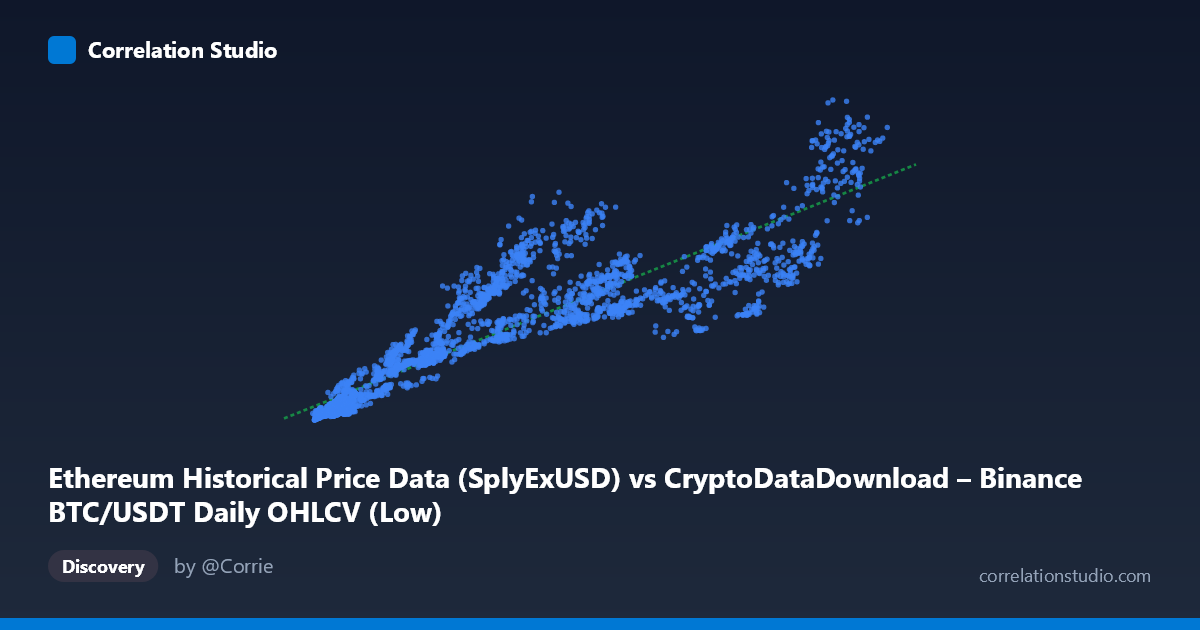
Ethereum Historical Price Data (SplyExUSD) vs CryptoDataDownload – Binance BTC/USDT Daily OHLCV (Low)
- Pearson correlation (r)
- 0.9043
- Spearman correlation
- 0.9431
- p-value
- 0
- Sample size (n)
- 3191
- 95% confidence interval
- 0.8978 to 0.9105
- Granger causality
- None
- Granger optimal lag
- 10
- Time coverage
- 2017-08-17 to 2026-05-20
AI analysis
Analysis of Ethereum Supply/Price Metric vs. Bitcoin Price Relationship
Note on labeling: The axis metadata appears inconsistent (X is labeled as an Ethereum supply metric while sample values resemble circulating supply units in the tens of thousands, and Y is labeled as BTC's daily low price in the tens of billions — an unusual magnitude for a single-coin price). Given the values, this is more plausibly a comparison of two large-scale, trending crypto market metrics (e.g., an ETH-related quantity vs. total BTC market value or similar aggregate). The analysis below treats the two series generically as X and Y, since the core statistical relationship is well-defined regardless of the exact metric confusion.
1. What the Visualization Reveals The scatterplot shows a strong, positive, roughly linear relationship between X and Y. As X increases from ~2,800 to ~123,000, Y climbs from ~1.4B to ~95.6B in a fairly consistent upward trend. The linear fit (y = 565,470x + 3.69B) tracks the data reasonably well across most of the range, though the sample points suggest some scatter/heteroscedasticity — particularly at low X values, where Y ranges from ~1.4B to ~20B despite similar X levels (e.g., X≈9,000–10,000 produces Y anywhere from 3.4B to 12.5B).
2. Strength, Direction, and Statistical Confidence The correlation coefficient (r = 0.904) indicates a strong positive linear relationship, with r² = 0.818 meaning 82% of the variance in Y is statistically explained by X — a substantial but not complete relationship, leaving ~18% of variance driven by other factors or noise. The 95% CI [0.898, 0.911] is tight, reflecting the large sample size (n=3,191) and giving high confidence that the true population correlation is robustly positive and strong. The p-value of ~0 confirms this correlation is highly unlikely to be due to chance.
However, the Granger causality tests are critical: neither direction (X→Y or Y→X) shows significant predictive causality (p = 0.82 and p = 0.79 respectively, even at an optimal lag of 10 periods). This means despite strong contemporaneous correlation, neither series helps forecast the other's future movements. This is a classic case of correlation without demonstrated temporal precedence — both variables likely move together due to a shared underlying driver (e.g., overall crypto market cycles, BTC dominance, or macro sentiment) rather than one causing the other.
3. Notable Patterns and Outliers - Low-X cluster variability: At small X values (under 10,000), Y shows considerable spread (3.4B–20B), suggesting a nonlinear or noisy relationship in this region — possibly an early-market phase with more volatility relative to the trend line. - High-X trend consistency: At larger X values (60,000), the relationship appears tighter and more linear, with Y scaling predictably. - Potential outlier: (35,440, 34.4B) stands out — Y is notably high relative to nearby X values like (34,757, 39.4B) and (30,200, 20.8B), indicating volatility or a regime shift at that point in time. - The overall shape suggests the relationship may not be perfectly linear across the full range — a log-log or power-law fit might improve explanatory power, especially given the wide range of both variables (X spans ~44x, Y spans ~67x).
4. Confounding Factors and Caveats Since both variables derive from cryptocurrency markets over a shared time period (2017–2026), they are both likely driven by common macro factors: overall crypto market capitalization cycles, Bitcoin dominance trends, regulatory news, and broad risk-on/risk-off sentiment. This shared temporal trend (both series generally rising over years) can inflate correlation through spurious trend correlation — two unrelated but co-trending time series will show high r even without genuine mechanistic linkage. The Granger causality null result reinforces this concern: the correlation is likely a byproduct of both series independently trending upward over the same multi-year bull/bear cycles, not a causal or predictive relationship.
5. Actionable Insights and Next Steps - Detrend or difference the data (e.g., analyze % daily/weekly changes instead of levels) to test whether the correlation persists after removing shared time trends — this will reveal if there's a genuine short-term relationship beneath the long-term co-movement. - Clarify the axis metadata — the current labels are ambiguous/contradictory (ETH supply vs. BTC price at mismatched scales), which should be resolved before drawing domain-specific conclusions. - Investigate the low-X volatility cluster and the (35,440, 34.4B) outlier via event-study analysis — check corresponding dates for market shocks or data anomalies. - Test nonlinear fits (log-log, polynomial) given the wide dynamic range of both variables to see if r² improves. - Given the lack of Granger causality, avoid using one series to forecast the other; instead, treat both as co-dependent outputs of a broader latent market factor (e.g., overall crypto market cap) and consider modeling that latent factor directly.
X dataset: CryptoDataDownload – Binance BTC/USDT Daily OHLCV
Y dataset: Ethereum Historical Price Data
Part of experiment: Bitcoin - CryptoDataDownload – Binance BTC/USDT Daily OHLCV vs Ethereum Historical Price Data