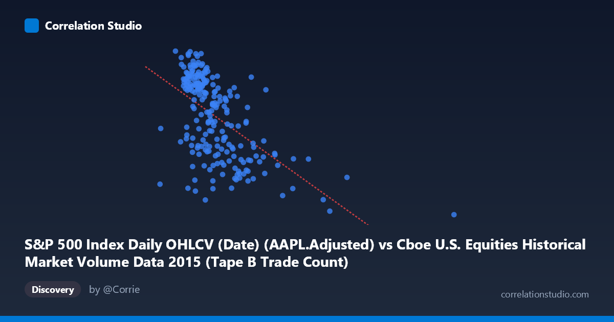
S&P 500 Index Daily OHLCV (Date) (AAPL.Adjusted) vs Cboe U.S. Equities Historical Market Volume Data 2015 (Tape B Trade Count)
- Pearson correlation (r)
- -0.5708
- Spearman correlation
- -0.5996
- p-value
- 0
- Sample size (n)
- 222
- 95% confidence interval
- -0.6534 to -0.4749
- Granger causality
- None
- Granger optimal lag
- 1
AI analysis
Analysis: AAPL Adjusted Price vs. Cboe Tape B Trade Count (2015)
Relationship Overview The scatterplot reveals a moderate negative relationship between Apple's adjusted stock price (X-axis) and the Cboe U.S. Equities Tape B trade count (Y-axis) across 2015. The linear regression equation (y = -4.04454E-05x + 128.804) indicates that as AAPL's adjusted price increases, Tape B trade counts tend to decline. This inverse pattern is visually apparent in the data, with lower price values clustering toward higher trade counts and higher price values associated with reduced trading activity on Tape B venues. The relationship, while statistically meaningful, is far from deterministic, with considerable scatter throughout the plot suggesting other forces are simultaneously at work.
Correlation Strength and Statistical Interpretation The Pearson correlation of r = -0.5708 indicates a moderate negative association. However, the coefficient of determination r² = 0.3259 is the more critical figure for practical interpretation — it means AAPL's adjusted price explains only about 32.6% of the variance in Tape B trade counts, leaving roughly 67.4% unexplained by this relationship alone. The 95% confidence interval of [-0.6534, -0.4749] is meaningfully narrow and does not cross zero, and the p-value of effectively 0 confirms this is not a chance finding given a sample of n = 222 from a population of 506. That said, statistical significance should not be conflated with practical significance — a 32.6% explained variance leaves substantial uncertainty. Critically, the Granger causality tests find no significant predictive directionality in either direction (X→Y: F = 1.27, p = 0.26; Y→X: F = 0.06, p = 0.81), meaning that past values of AAPL price do not reliably predict future Tape B trade counts, and vice versa. The correlation is contemporaneous rather than temporally predictive.
Notable Patterns, Clusters, and Outliers The bulk of the data concentrates in the X range of roughly 200,000–400,000, where Tape B trade counts span widely from approximately 105 to 128 — suggesting high variability in trade counts even at similar price levels. Two prominent high-leverage outliers are visible: one near (1,014,194, 100.01) and another near (640,679, 100.61), both sitting far to the right with very low trade counts. These extreme observations almost certainly exert disproportionate influence on the regression slope and correlation coefficient. There also appears to be a mild clustering of high trade counts (122–128) at lower price levels (~200,000–260,000), potentially reflecting a period earlier in 2015 when AAPL traded at lower adjusted values and Tape B activity was elevated. A subtle non-linear or heteroscedastic pattern may be present — variance in Y appears to compress at higher X values, hinting that a log transformation or non-linear model might better characterize the true relationship.
Confounding Factors and Caveats Several important caveats temper interpretation. First, the axis labels appear to be swapped or counterintuitive — the X-axis is labeled as AAPL adjusted price but has a range (130,085–1,014,194) that resembles a volume or trade count scale rather than a stock price, while the Y-axis labeled as Tape B trade count has values (100–128) more consistent with a stock price range. This dataset-column assignment warrants careful verification before drawing conclusions. Second, the time period (February–December 2015) was marked by notable market volatility, including the August 2015 correction, which could simultaneously depress prices and alter trading venue preferences. Third, market structure shifts — such as changes in Tape B-listed ETF activity, routing practices, or intraday volume patterns — could independently drive both variables, creating a spurious or partially confounded correlation. The absence of Granger causality further supports the idea that this is a coincident rather than causal relationship.
Actionable Insights and Further Investigation Given the moderate correlation, partial explanatory power, and absence of Granger causality, this relationship should not be used as a predictive trading signal. However, several follow-up analyses are warranted: (1) Verify and potentially correct the axis/column assignments to ensure the relationship being modeled is as intended. (2) Investigate the two extreme outliers — identifying their specific dates may reveal event-driven anomalies (e.g., expiration dates, macro announcements) that disproportionately shape the correlation. (3) Apply a log transformation to the X variable to address the right-skewed distribution and potential heteroscedasticity. (4) Introduce multivariate regression incorporating broader market volume (VIX, SPX volume, or total market trade counts) to better isolate whether AAPL price has any independent relationship with Tape B activity after controlling for market-wide conditions. (5) Segment the analysis by sub-period (pre- and post-August correction) to assess whether the observed correlation is consistent across the year or driven by a specific market regime.
X dataset: Cboe U.S. Equities Historical Market Volume Data 2015
Y dataset: S&P 500 Index Daily OHLCV (Date)
Part of experiment: Daily - Cboe U.S. Equities Historical Market Volume Data 2015 vs S&P 500 Index Daily OHLCV (Date)