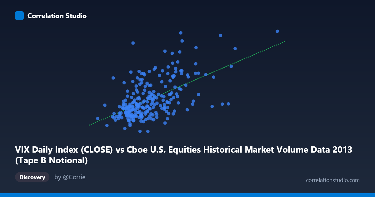
VIX Daily Index (CLOSE) vs Cboe U.S. Equities Historical Market Volume Data 2013 (Tape B Notional)

Pearson correlation (r): 0.5669
Spearman correlation: 0.5245
p-value: 0
Sample size (n): 252
95% confidence interval: 0.4768 to 0.6453
Granger causality: None
Granger optimal lag: 1

AI analysis

Scatterplot Analysis: VIX Daily Index vs. Tape B Notional Volume (2013)

1. Overall Relationship The scatterplot reveals a moderate positive relationship between the VIX Daily Index (CLOSE) and Tape B Notional trading volume across U.S. equity exchanges in 2013. As the VIX rises — indicating greater market fear or uncertainty — Tape B Notional volume tends to increase as well. This is consistent with well-established market intuition: heightened volatility typically drives elevated trading activity as investors reposition, hedge, or react to news. The linear regression equation (y = 9.41e-10x + 10.58) confirms a positive slope, though the intercept suggests a meaningful baseline volume exists even at low VIX levels.

2. Correlation Strength and Statistical Significance The correlation coefficient of r = 0.5669 indicates a moderate positive association. However, r² = 0.3214 means that only about 32% of the variance in Tape B Notional volume is explained by VIX levels, leaving roughly 68% attributable to other factors. The 95% confidence interval for r of [0.4768, 0.6453] is reasonably tight and excludes zero, and the p-value of essentially 0 confirms the relationship is highly statistically significant across the sample of 252 paired observations drawn from a population of 3,780. That said, statistical significance here should not be confused with practical determinism — the explained variance is modest at best. Critically, Granger causality tests in both directions (X→Y: F=0.63, p=0.43; Y→X: F=0.61, p=0.44) fail to reach significance, meaning neither variable reliably predicts the other in a temporal, lead-lag sense at the one-period lag tested. The relationship appears contemporaneous rather than directionally predictive.

3. Notable Patterns, Clusters, and Outliers The data points show a broad, dispersed cloud concentrated in the VIX range of roughly 2.5–5.5 billion (on the X-axis scale) and Y values between 12 and 17, suggesting the bulk of 2013 trading days were characterized by moderate volatility and moderate Tape B activity. Several notable outliers are visible: the point near (5.19B, 20.34) stands out as a high-volume, high-VIX day, likely corresponding to a specific market stress event. Similarly, observations like (7.30B, 17.27) and (6.56B, 16.28) represent unusually high VIX readings that still produced only mid-range Tape B notional values, suggesting diminishing returns or nonlinearity at the upper tail. There is also visible heteroscedasticity — the spread of Y values widens noticeably as X increases — implying the relationship is less predictable during high-volatility regimes.

4. Confounding Factors and Caveats Several important caveats apply. First, Tape B Notional volume aggregates trading across NYSE American-listed securities, which may respond to sector-specific drivers unrelated to broad market volatility as captured by VIX. Second, 2013 was a particularly low-volatility, bull-market year (VIX averaged historically low levels), which compresses the dynamic range of the relationship and may limit generalizability. Third, day-of-week effects, macroeconomic announcements, earnings seasons, and Federal Reserve communications all influence both VIX and notional volume simultaneously, creating classic confounding. The failure of Granger causality also warns against assuming any mechanistic link — the correlation may reflect shared responses to common shocks rather than any direct causal pathway. Finally, the mismatch in dataset labeling (X and Y axes appear swapped from their source dataset descriptions) warrants verification before drawing firm conclusions.

5. Actionable Insights and Further Investigation Practitioners should avoid using VIX alone as a reliable predictor of Tape B Notional volume for trading or risk management purposes, given that only ~32% of variance is explained and no temporal predictive direction is established. Further investigation should test nonlinear model forms (e.g., log-log or polynomial regression) to address the apparent heteroscedasticity and potential curvature in the relationship. Expanding the Granger causality analysis to multiple lags (2–5 periods) could uncover delayed relationships not visible at lag 1. Analysts should also condition the analysis on volatility regimes (e.g., VIX above/below 20) to assess whether the correlation strengthens during stress periods. Finally, incorporating additional explanatory variables — such as S&P 500 returns, news sentiment indices, or options expiration calendars — into a multivariate framework would substantially improve explanatory power and provide more actionable forecasting capability.

X dataset: Cboe U.S. Equities Historical Market Volume Data 2013

Y dataset: VIX Daily Index

Part of experiment: Daily - Cboe U.S. Equities Historical Market Volume Data 2013 vs VIX Daily Index