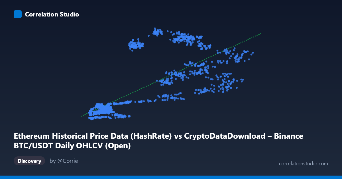
Ethereum Historical Price Data (HashRate) vs CryptoDataDownload – Binance BTC/USDT Daily OHLCV (Open)
- Pearson correlation (r)
- 0.7515
- Spearman correlation
- 0.7567
- p-value
- 0
- Sample size (n)
- 1855
- 95% confidence interval
- 0.731 to 0.7706
- Granger causality
- None
- Granger optimal lag
- 1
AI analysis
Scatterplot Analysis: Ethereum Hash Rate (X) vs. BTC/USDT Open Price (Y)
1. What the Visualization Reveals
The scatterplot shows a positive, moderately strong relationship between the X-variable (labeled as Ethereum hash rate, though the mislabeled column header suggests this may actually be a BTC-related metric given the dataset descriptions) and the Y-variable (BTC/USDT opening price). As X increases from roughly 3,000 to 67,000, Y generally trends upward from double digits to four-digit values. However, the relationship is far from a tight line — there's substantial vertical scatter at almost every X level, particularly in the 8,000–13,000 range where Y values span from ~104 to ~243, and again in the 20,000–50,000 range where Y ranges from ~269 to over 1,000.
2. Strength, Direction, and Uncertainty
The correlation coefficient (r = 0.7515) indicates a strong positive linear relationship, but the r² of 0.5647 tells the more practically important story: only 56.5% of the variance in Y is explained by X, leaving nearly 44% attributable to other factors, noise, or non-linear dynamics. The 95% confidence interval [0.731, 0.771] is tight, and the p-value of ~0 confirms this correlation is highly statistically significant — it is not a chance artifact given the large sample (n=1,855). However, statistical significance should not be conflated with strong predictive power; r² caps how much confidence we should place in X as a standalone predictor of Y.
Critically, the Granger causality tests show no significant predictive direction in either direction (X→Y: p=0.264; Y→X: p=0.474). This means that past values of one series do not significantly help forecast future values of the other beyond what the series' own history provides. This is an important caveat: despite the strong contemporaneous correlation, there is no evidence of a lead-lag temporal relationship at the tested lag (1 period). This strongly suggests the correlation is driven by a shared underlying trend or co-movement (e.g., both series rising over the 2017–2022 crypto bull/bear cycles) rather than one variable causally driving the other over time.
3. Notable Patterns and Outliers
Several structural features stand out: - Low-X cluster (X < 15,000): Y values are tightly bunched between ~100–250, suggesting a compressed, low-variance regime — likely corresponding to earlier/bearish market periods. - Mid-to-high-X scatter (X = 20,000–50,000): This region shows the widest dispersion, with Y ranging from ~269 to over 1,000 at similar X values (e.g., X≈20,287 → Y≈896 vs. X≈23,107 → Y≈269). This heteroskedasticity suggests the relationship is not uniform across the range and may reflect distinct market regimes or a non-linear (possibly logarithmic or regime-switching) relationship rather than a simple linear one. - High-X tail (X 50,000): Fewer points here show moderate Y values (438–715), potentially indicating diminishing returns or a plateau effect at higher X.
4. Confounding Factors and Caveats
The most significant caveat is the apparent data labeling inconsistency — the X-axis is described as an Ethereum hash rate metric pulled from a BTC/USDT OHLCV dataset, while Y is explicitly BTC/USDT open price. This mismatch suggests possible metadata/column-mapping errors that should be verified before drawing conclusions. Beyond this, both cryptocurrencies are known to be highly correlated due to shared macro drivers (overall crypto market sentiment, Bitcoin dominance effects, regulatory news, and correlated retail/institutional flows) rather than a direct mechanical link between hash rate and price. Time itself is a likely confounder: both series may simply trend upward together over the 2017–2022 window due to overall market growth, inflating the correlation without implying direct causation (classic spurious correlation via a common trend).
5. Suggestions for Further Investigation
1. Verify column mapping — confirm whether X truly represents hash rate or was mislabeled, given the dataset descriptions point to BTC price data on both axes. 2. Detrend or difference the series (e.g., use returns/percentage changes instead of levels) before re-testing correlation and Granger causality, since price and hash rate series are typically non-stationary and prone to spurious correlation in levels. 3. Segment by market regime (bull vs. bear periods) to see if the relationship strength or slope changes — the observed heteroskedasticity hints at regime-dependent behavior. 4. Test additional lags in Granger causality (beyond lag 1) and consider higher-frequency data, since crypto markets can have causal effects that manifest over hours/days rather than single-period lags. 5. Introduce a third variable (e.g., overall crypto market cap, BTC network hash rate, or macro liquidity indicators) to test whether the X-Y correlation is mediated or spurious.
X dataset: CryptoDataDownload – Binance BTC/USDT Daily OHLCV
Y dataset: Ethereum Historical Price Data
Part of experiment: Bitcoin - CryptoDataDownload – Binance BTC/USDT Daily OHLCV vs Ethereum Historical Price Data