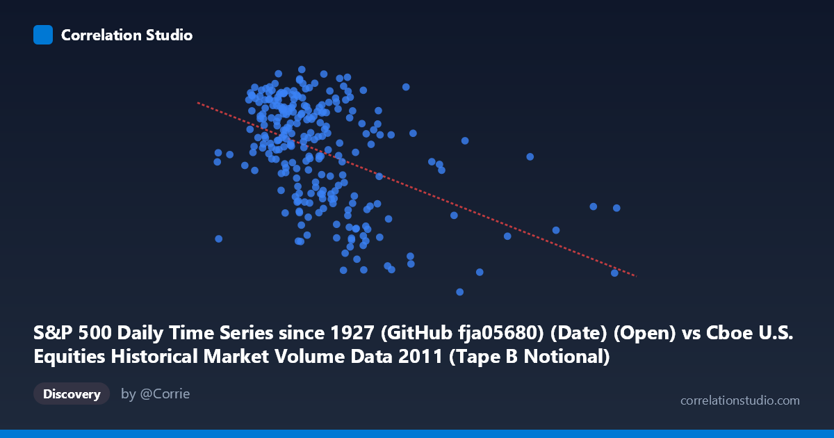
S&P 500 Daily Time Series since 1927 (GitHub fja05680) (Date) (Open) vs Cboe U.S. Equities Historical Market Volume Data 2011 (Tape B Notional)
- Pearson correlation (r)
- -0.4552
- Spearman correlation
- -0.4251
- p-value
- 0
- Sample size (n)
- 252
- 95% confidence interval
- -0.548 to -0.3514
- Granger causality
- None
- Granger optimal lag
- 4
AI analysis
Analysis: S&P 500 Open Price vs. Cboe Tape B Notional Volume (2011)
Relationship Overview
The scatterplot reveals a moderate negative relationship between the S&P 500 daily open price (X-axis, expressed as a date serial/timestamp value) and Cboe Tape B Notional trading volume (Y-axis). As time progresses through 2011, Tape B Notional volume tends to decline. The linear regression equation (y = -1.584×10⁻⁸x + 1348.58) confirms this downward trajectory, though the relationship is far from deterministic. The data spans 252 trading days in 2011, drawn from a population of 3,780 observations, giving reasonable statistical power to detect this trend.
Correlation Strength and Statistical Significance
The Pearson correlation of r = -0.4552 indicates a moderate negative association, but the more practically important metric is r² = 0.2072, meaning only about 20.7% of the variance in Tape B Notional volume is explained by the temporal position (S&P 500 date encoding). The remaining ~79% is driven by other factors entirely. The 95% confidence interval of [-0.548, -0.351] is entirely negative and does not include zero, reinforcing directional confidence, and the p-value of 2.71×10⁻¹⁴ confirms this is highly unlikely to be a chance finding. However, statistical significance here is partly a function of the large sample size (N=3,780), so practical significance deserves independent scrutiny. Critically, the Granger causality test found no significant predictive direction in either direction (X→Y: F=2.03, p=0.092; Y→X: F=0.27, p=0.896), meaning that even though a contemporaneous correlation exists, neither variable reliably predicts the other's future values at the optimal 4-period lag. This is an important caveat: the relationship is associative and temporal, not mechanistically predictive.
Notable Patterns, Clusters, and Outliers
Several features stand out in the sample points. There are clear outliers on the high-X (late-year) end — points near X = 9.5–14.1 billion (representing later dates in 2011) that show a wide spread of Y values, suggesting increased volatility or structural breaks in market volume during that period. Notably, points like (9,956,196,749; 1121.30) and (8,812,375,572; 1243.97) represent substantially depressed Tape B Notional values compared to mid-year observations, pulling the regression slope downward. Conversely, mid-range X values (roughly 3.0–5.5 billion range) show a dense cluster with relatively high and variable Y values (1,270–1,365), suggesting that earlier in 2011, Tape B volume was both higher on average and more variable. The spread of Y values across all X ranges also hints at heteroscedasticity — variance in Y appears to decrease slightly at higher X values, which would violate standard OLS assumptions.
Confounding Factors and Caveats
Several important caveats apply. First, the X-axis encodes dates as numeric timestamps, so this correlation is fundamentally a time trend analysis, not a direct causal relationship between S&P 500 price levels and trading volume. The declining Tape B Notional volume through 2011 likely reflects broader structural changes — including the August 2011 market volatility spike (debt ceiling crisis, U.S. credit downgrade), seasonal trading patterns, and ongoing shifts in exchange market share between Cboe tapes (A, B, C). Second, Tape B specifically covers NYSE MKT and regional exchange listings, so its volume dynamics may reflect exchange competition and routing changes rather than pure market-level activity. Third, using daily open prices as a date proxy is methodologically imprecise; a simple integer day index would be cleaner for trend analysis.
Actionable Insights and Further Investigation
Given these findings, several investigations would add value. Decomposing the 2011 time series into distinct regimes — pre- and post-August volatility event — would likely reveal that the correlation is driven heavily by that structural break rather than a smooth secular trend. Comparing Tape A, B, and C Notional volumes simultaneously would clarify whether this is a Tape B-specific phenomenon or a market-wide volume decline. Analysts should also test non-linear models (e.g., piecewise regression or LOESS smoothing), given the visible heteroscedasticity and the relatively weak linear fit. Finally, incorporating VIX or S&P 500 realized volatility as a covariate would help disentangle whether the volume decline reflects lower volatility regimes rather than a pure time trend, which would be the more actionable insight for trading or market structure research.
X dataset: Cboe U.S. Equities Historical Market Volume Data 2011
Y dataset: S&P 500 Daily Time Series since 1927 (GitHub fja05680) (Date)
Part of experiment: Daily - Cboe U.S. Equities Historical Market Volume Data 2011 vs S&P 500 Daily Time Series since 1927 (GitHub fja05680) (Date)