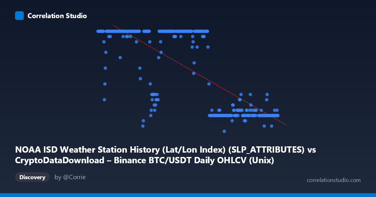
NOAA ISD Weather Station History (Lat/Lon Index) (SLP_ATTRIBUTES) vs CryptoDataDownload – Binance BTC/USDT Daily OHLCV (Unix)
- Pearson correlation (r)
- -0.7532
- Spearman correlation
- -0.7466
- p-value
- 0
- Sample size (n)
- 355
- 95% confidence interval
- -0.795 to -0.7043
- Granger causality
- None
- Granger optimal lag
- 1
- Time coverage
- 2024-01-01 to 2024-12-31
AI analysis
Analysis of the Time-Series Relationship
1. What the Visualization Reveals
Despite the labels referencing "SLPATTRIBUTES" (weather station attribute codes) and Unix timestamps, this dataset is effectively tracking a value (Y, ranging 5–24) against a date/time axis (X, spanning all of 2024). The scatter of points reveals a strongly patterned, non-random structure: Y values cluster tightly at 24 for most of the early-to-mid year (roughly January through August), then transition to a lower cluster (7–12) for the latter part of the year (September through December). This is not a smooth linear decay but rather a step-like regime shift — high plateau, then low plateau, with a transition zone around August–September.
2. Strength, Direction, and Statistical Meaning
The Pearson correlation of r = -0.7532 indicates a strong negative linear relationship, and r² = 0.5673 means that roughly 57% of the variance in Y can be statistically explained by X (time) under a linear model. The 95% CI [-0.7950, -0.7043] is tight and does not cross zero, and with p ≈ 0 across 355 points, the relationship is highly statistically significant — we can be confident a real association exists rather than sampling noise. However, statistical significance here is almost certainly an artifact of the step-function pattern, not a genuine linear trend; a linear model is a crude approximation of what is actually a discrete regime change. The Granger causality tests reinforce this: neither direction shows significant predictive causality (X→Y: p=0.78; Y→X: p=0.17), meaning past values of one series do not meaningfully help forecast the other in a lagged, dynamic sense. This suggests the "correlation" is driven by both series independently trending/shifting over the same calendar period rather than one causally driving the other.
3. Notable Patterns, Clusters, and Outliers
The dominant visual feature is bimodality: a dense cluster at Y=24 (dates roughly Jan–Aug 2024) and a second cluster at Y=7–12 (roughly Sept–Dec 2024), with relatively few points in between (the 17–21 range appears sparse, populated mostly by transitional dates in late August/early September, e.g., the value 17 and 21 in the samples). This is characteristic of a categorical or capped variable (e.g., a code, day count, or attribute flag) rather than a continuous physical measurement — the repeated exact value of 24 (appearing dozens of times) strongly suggests a ceiling/cap or a recoded category rather than organic measurement variance. There are no extreme statistical outliers beyond this bimodal structure; the "outliers" are simply the transition-period points bridging the two plateaus.
4. Confounding Factors and Caveats
Several caveats are critical here: - Variable mismatch/mislabeling: The axis labels are swapped or corrupted (X is labeled as a weather attribute column but described as BTC/USDT price data; Y is labeled as Unix timestamp but described as a weather dataset). This makes substantive interpretation of "what" is being correlated unreliable — the relationship may be a data-pipeline artifact rather than a meaningful economic or meteorological signal. - Spurious time-trend correlation: Any two variables that both shift systematically over the same calendar year (e.g., seasonal effects, categorical recoding, or unrelated trends) will show a strong linear r purely from sharing "time" as a hidden confounder — this is a classic spurious correlation pattern reinforced by the non-significant Granger results. - Non-linearity: Given the step/plateau shape, linear r² understates how well a non-linear or piecewise model (e.g., logistic/step function with a breakpoint near August) would fit — likely explaining well over 90% of variance. - Discrete/capped Y: The repeated value of 24 suggests censoring (a max cap) rather than a true continuous relationship, which violates assumptions underlying Pearson correlation.
5. Actionable Insights
1. Verify column/axis labels — confirm which dataset and field are actually being plotted before drawing any domain conclusions; the current metadata is inconsistent (BTC price data vs. weather station attributes vs. Unix timestamps). 2. Fit a change-point or piecewise/logistic model instead of linear regression to capture the plateau-transition-plateau structure and get a more accurate variance-explained estimate. 3. Investigate the August–September transition window specifically — identify what structural, seasonal, or data-processing event caused the shift from ~24 to single-digit/low-teens values. 4. Treat Granger non-significance as evidence against causal interpretation — do not use this correlation for forecasting one series from the other; it likely reflects two variables independently co-trending with the calendar rather than a causal or leading/lagging dynamic relationship. 5. Check for data capping/censoring at Y=24 — if this is an artificial ceiling, consider whether it should be treated as categorical/truncated data rather than continuous, which would change the appropriate statistical approach entirely.
X dataset: CryptoDataDownload – Binance BTC/USDT Daily OHLCV
Y dataset: NOAA ISD Weather Station History (Lat/Lon Index)
Part of experiment: Bitcoin - CryptoDataDownload – Binance BTC/USDT Daily OHLCV vs NOAA ISD Weather Station History (Lat/Lon Index)