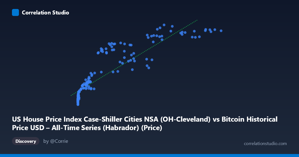
US House Price Index Case-Shiller Cities NSA (OH-Cleveland) vs Bitcoin Historical Price USD – All-Time Series (Habrador) (Price)
- Pearson correlation (r)
- 0.8936
- Spearman correlation
- 0.9645
- p-value
- 0
- Sample size (n)
- 191
- 95% confidence interval
- 0.8609 to 0.919
- Granger causality
- None
- Granger optimal lag
- 2
- Time coverage
- 2010-08-01 to 2026-06-01
- Recomputed on refreshed data
- 2026-10-24 (r was 0.8898)
AI analysis
Analysis: Bitcoin Price vs. Case-Shiller Home Price Index (Cleveland)
1. What the Visualization Reveals
The scatterplot shows a strong positive association between Bitcoin's historical USD price (X-axis) and the Case-Shiller Cleveland home price index (Y-axis). However, the relationship is clearly non-linear — the data traces a curve rather than a straight line. At low Bitcoin prices (under ~$1,000), the home price index clusters tightly between 95-115, showing little sensitivity to X. As Bitcoin prices climb into the tens of thousands, the index rises more steeply and then appears to plateau/saturate around 195-205 at the highest Bitcoin prices ($85,000). This resembles a logarithmic or saturating growth curve rather than a proportional linear relationship.
2. Strength, Direction, and Practical Meaning
The correlation coefficient (r = 0.887) indicates a strong positive linear relationship, with r² = 0.787 meaning the linear model explains about 79% of the variance in Y. The 95% CI [0.852, 0.914] is tight and the p-value is effectively 0, so the correlation itself is highly statistically robust — this is not a fluke of sampling. However, statistical significance of correlation does not imply causation. The Granger causality tests are decisive here: neither direction shows significant predictive causality (X→Y: p=0.193; Y→X: p=0.112). This strongly suggests the observed correlation is not driven by one variable temporally leading the other, but rather both series are likely responding to a shared underlying driver (e.g., time itself, or macroeconomic conditions like monetary expansion, low interest rates, and general asset inflation over the 2010–2026 period).
3. Notable Patterns and Outliers
- Compressed low-end cluster: Dozens of points with X < 1,000 show Y tightly bound between 94-115, indicating Bitcoin's early years (2010-2013) coincided with a relatively flat, slow-recovering housing market post-2008 crash. - Steep-then-flat mid/high range: Between X ≈ 20,000–60,000, Y climbs rapidly (120→195), but beyond X ≈ 85,000, Y plateaus near 195-205, suggesting a ceiling effect — house prices don't scale with Bitcoin's later exponential rallies. - Scale mismatch: X spans nearly 6 orders of magnitude (0.06 to 118,670) while Y varies only about 2-fold (94 to 204). This extreme heteroscedasticity in scale is a hallmark of two series growing at very different rates, both merely trending upward over time.
4. Confounding Factors and Caveats
The most significant caveat: this is very likely a spurious/co-integrated time-trend correlation. Both Bitcoin price and home price indices have exhibited long-term upward trends over the 2010–2026 window independent of each other — Bitcoin due to adoption/speculation cycles, and home prices due to demographic demand, low interest rates, and general inflation. Any two non-stationary time series with upward trends will show high correlation without genuine mechanistic linkage. The lack of Granger causality in either direction reinforces that time (or a common macro factor like Fed policy/inflation/liquidity) is the true confound, not a direct economic relationship between crypto markets and Cleveland real estate.
5. Suggestions for Further Investigation
- De-trend both series (e.g., using year-over-year % changes or differencing) and re-test correlation on the detrended/stationary series to see if the relationship survives — likely it will weaken substantially. - Introduce a common macro covariate (M2 money supply, federal funds rate, CPI) to test if both series are jointly explained by shared monetary conditions. - Test non-linear/log models: given the visible saturation curve, a log(X) or logistic fit likely outperforms the linear model (R²=0.787) and may better characterize the true functional relationship. - Treat this correlation as descriptive/coincidental rather than predictive; it should not be used for forecasting one asset from the other given the null Granger causality results.
X dataset: Bitcoin Historical Price USD – All-Time Series (Habrador)
Y dataset: US House Price Index Case-Shiller Cities NSA
Part of experiment: Bitcoin - Bitcoin Historical Price USD – All-Time Series (Habrador) vs US House Price Index Case-Shiller Cities NSA