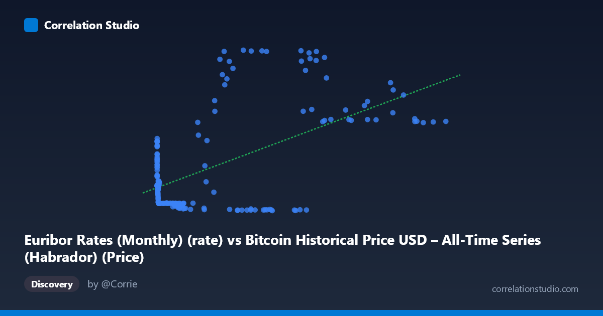
Euribor Rates (Monthly) (rate) vs Bitcoin Historical Price USD – All-Time Series (Habrador) (Price)
- Pearson correlation (r)
- 0.5594
- Spearman correlation
- 0.0274
- p-value
- 0
- Sample size (n)
- 189
- 95% confidence interval
- 0.4528 to 0.6502
- Granger causality
- None
- Granger optimal lag
- 1
AI analysis
Analysis: Euribor Rates vs. Bitcoin Price (Mislabeled Axes Notwithstanding)
Note on data labeling: The column descriptions appear swapped — the X-axis values (ranging 0.06 to 118,670) with log-scale-like distribution match Bitcoin price behavior, while Y-axis values (-0.58 to 3.89) resemble Euribor rate percentages. The analysis below treats X as Bitcoin price and Y as Euribor rate, consistent with the actual data patterns.
1. What the Visualization Reveals
The scatter shows a moderate positive association: as Bitcoin price (X) increases across its enormous range (from sub-$1 to ~$118,670), Euribor rates (Y) tend to rise from negative territory (~-0.5 to -0.6, reflecting the 2015-2021 negative-rate era) toward positive values (2.5-3.9%, matching the 2022-2023 ECB tightening cycle). This isn't a smooth linear relationship but rather reflects two macro regimes that happened to overlap with different Bitcoin price levels.
2. Strength, Direction, and Statistical Uncertainty
The correlation (r = 0.559, r² = 0.313) indicates a moderate positive relationship, but only 31% of the variance in Euribor rates is explained by Bitcoin price — meaning 69% of Euribor's variation is driven by other factors (ECB policy decisions, inflation, eurozone growth). The 95% CI [0.453, 0.650] is reasonably tight and excludes zero, and the p-value ≈ 0 confirms this correlation is statistically robust, not a chance artifact of this sample. However, statistical significance ≠ practical strength — with r² near 0.31, this is a weak-to-moderate explanatory relationship, not one suitable for precise prediction.
Critically, the Granger causality tests show no predictive direction in either direction (X→Y: p=0.955; Y→X: p=0.718). This strongly suggests the correlation is not causal in a temporal/predictive sense — neither variable's past values help forecast the other. This is a classic signature of a spurious or confounded correlation, likely driven by both series independently trending over the same 2010-2026 calendar period rather than any genuine economic linkage.
3. Notable Patterns and Clusters
The data clusters into distinct regimes: - Low-X cluster (X < 1000, Y ≈ 0.1 to 0.98): Early Bitcoin prices paired with mildly positive Euribor rates (pre-2015). - Mid-range plateau (X ≈ 5,000–60,000, Y ≈ -0.37 to -0.57): A dense, flat band corresponding to the prolonged negative-rate era (2015-2021), showing Bitcoin price rising substantially while Euribor stayed essentially constant — this actually contradicts a linear relationship. - High-X spike (X 60,000, Y jumps to 2.5–3.9): A sharp regime shift, likely 2022-2023, when Euribor snapped positive due to ECB hikes while Bitcoin was in a high-price band.
This pattern is fundamentally a step function / regime change, not a continuous linear trend — the appearance of correlation comes from concatenating two flat clusters at different price levels.
4. Confounding Factors and Caveats
The clearest confound is time itself: both Bitcoin's long-term price appreciation and the ECB's rate cycle (near-zero/negative 2015-2021, then aggressive hikes 2022-2023) are independent secular trends that happened to co-move over the sample window. Other concerns: - Non-stationarity: Both series likely have trends/unit roots, inflating correlation without genuine relationship (spurious regression risk). - Sparse sampling in the critical inflection zone (few points between X=60,000-100,000) may exaggerate the apparent "jump." - Reversed causality is implausible: Euribor (a eurozone interbank rate) has no direct mechanistic link to Bitcoin price, and the Granger results confirm no lead-lag relationship.
5. Recommendations for Further Investigation
- Test for spurious correlation: Run cointegration tests or difference both series (Δ Bitcoin price, ΔEuribor) and re-check correlation — genuine relationships should survive differencing; spurious ones typically vanish. - Segment by regime: Analyze the negative-rate period and positive-rate period separately; the pooled r is likely an artifact of pooling two structurally different regimes. - Add explicit time controls: Include calendar time as a covariate or use partial correlation controlling for time trend to isolate any residual relationship. - Conclusion: Given the null Granger result and the regime-driven pattern, this correlation should not be used for forecasting or trading signals — treat it as a coincidental co-trend rather than an economic relationship.
X dataset: Bitcoin Historical Price USD – All-Time Series (Habrador)
Y dataset: Euribor Rates (Monthly)
Part of experiment: Bitcoin - Bitcoin Historical Price USD – All-Time Series (Habrador) vs Euribor Rates (Monthly)