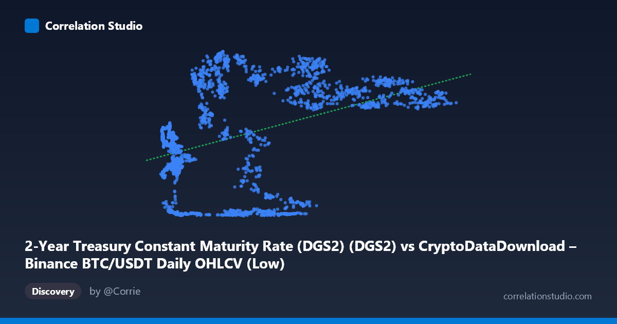
2-Year Treasury Constant Maturity Rate (DGS2) (DGS2) vs CryptoDataDownload – Binance BTC/USDT Daily OHLCV (Low)
- Pearson correlation (r)
- 0.4023
- Spearman correlation
- 0.3898
- p-value
- 0
- Sample size (n)
- 2197
- 95% confidence interval
- 0.3666 to 0.4368
- Granger causality
- None
- Granger optimal lag
- 1
AI analysis
Analysis: BTC/USDT (X) vs. 2-Year Treasury Yield (Y)
Note on axis labeling: The metadata appears mislabeled — the X-axis values (2,817–123,084) are clearly BTC/USDT prices, while the Y-axis values (0.09–5.19) match 2-Year Treasury yields. I'll proceed with this corrected interpretation, treating X = BTC price and Y = DGS2 yield.
1. What the Visualization Reveals
The scatterplot shows a weak-to-moderate positive relationship between Bitcoin price and the 2-year Treasury yield. Rather than a clean linear trend, the data appears to cluster into distinct regimes: a low-price/low-yield cluster (BTC below ~50,000, yields near 0.1–0.3, likely reflecting the near-zero rate environment of 2020–2021) and a higher-price/higher-yield cluster (BTC above ~40,000–120,000, yields clustering around 3.5–5.0, reflecting the 2022–2024 rate-hiking cycle). This bimodal clustering — rather than a smooth continuous relationship — is likely the primary driver of the measured correlation.
2. Strength, Direction, and Statistical Confidence
The correlation coefficient (r = 0.402) indicates a weak positive linear relationship, with r² = 0.162 meaning only about 16% of the variance in Treasury yields is explained by BTC price (or vice versa) — leaving 84% unexplained by this simple linear relationship. The 95% CI [0.367, 0.437] is fairly tight given the large sample size (n=2,197), and the p-value of ~0 confirms the correlation is statistically significant and not due to chance. However, statistical significance with such a large n is expected even for modest effect sizes — the practical significance is limited by the low r². Critically, the Granger causality tests show no significant predictive direction in either direction (X→Y: p=0.132; Y→X: p=0.400), indicating that neither series reliably helps forecast the other's short-term (1-lag) movements. This strongly suggests the correlation is not driven by direct causal or lead-lag dynamics but rather reflects both variables independently trending over a shared macro period.
3. Notable Patterns and Outliers
The data shows clear non-linear/regime-based structure rather than a single linear trend: - A dense low-yield cluster (Y < 1.0) spanning a wide range of BTC prices (7,000–57,000), representing the 2020–2021 near-zero rate era. - A dense high-yield cluster (Y = 3.5–5.0) also spanning a wide BTC range (16,000–120,000), representing 2022 onward. - Notable outliers include points like (6,380, 2.56) and (7,076, 1.72) — low BTC prices paired with mid-range yields — which don't fit either dominant cluster and may reflect transitional periods (rate hikes beginning while BTC was still depressed, e.g., early 2022).
This clustering pattern means the linear regression line (y = 2.02×10⁻⁵x + 1.875) is a poor descriptor of the actual relationship; the true structure is closer to a step-function or regime-shift pattern than a continuous linear one.
4. Confounding Factors and Caveats
The most important caveat is that this is a classic case of spurious/confounded correlation via time. Both series are time-ordered (2017–2026) and both underwent major independent regime shifts driven by the same macro backdrop (Fed policy pivots, COVID-era stimulus, 2022 inflation-driven hikes, subsequent crypto bull market). Correlating two non-stationary trending time series without differencing or detrending commonly inflates apparent correlation even when no direct mechanistic link exists. Additionally, N (3,212) vs. n (2,197) suggests substantial missing/unpaired data, which could introduce sampling bias if data gaps aren't random (e.g., missing Treasury data on holidays vs. continuous crypto trading).
5. Suggestions for Further Investigation
1. Detrend or difference both series (e.g., use daily/weekly returns rather than levels) and recompute correlation — this will reveal whether any relationship survives once shared macro trends are removed. 2. Segment by regime (pre/post 2022 hiking cycle) and analyze correlations within each period separately, since pooling regimes likely inflates r artificially. 3. Test longer Granger lags (weekly/monthly) since 1-day lag may be too short to capture monetary policy transmission effects on risk assets. 4. Incorporate additional variables (e.g., DXY, real yields, Fed funds rate, equity indices) to test whether BTC's relationship with rates is direct or mediated through broader risk-asset/liquidity conditions. 5. Treat this correlation as descriptive/historical co-movement, not predictive or causal — it should not be used for trading signals given the null Granger results.
X dataset: CryptoDataDownload – Binance BTC/USDT Daily OHLCV
Y dataset: 2-Year Treasury Constant Maturity Rate (DGS2)
Part of experiment: Bitcoin - CryptoDataDownload – Binance BTC/USDT Daily OHLCV vs 2-Year Treasury Constant Maturity Rate (DGS2)