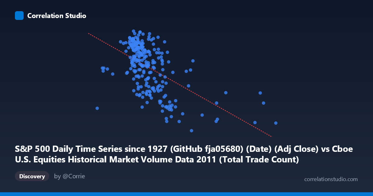
S&P 500 Daily Time Series since 1927 (GitHub fja05680) (Date) (Adj Close) vs Cboe U.S. Equities Historical Market Volume Data 2011 (Total Trade Count)

Pearson correlation (r): -0.5534
Spearman correlation: -0.5499
p-value: 0
Sample size (n): 252
95% confidence interval: -0.6336 to -0.4614
Granger causality: None
Granger optimal lag: 1

AI analysis

Analysis: S&P 500 Price vs. U.S. Equities Total Trade Count (2011)

Relationship Overview The scatterplot reveals a moderate negative relationship between S&P 500 adjusted closing prices (X-axis) and total trade counts across U.S. equity exchanges (Y-axis) during 2011. As the S&P 500 price level rises, total trade count tends to decrease, and conversely, lower price levels correspond with higher trading activity. The linear regression equation (y = -6.46e-05x + 1,398.39) quantifies this inverse relationship, suggesting that for every ~15,500-point increase in the S&P 500 index, trade count drops by roughly 1 unit on the scale used. The data spans the full 2011 calendar year across 252 paired observations drawn from a population of 3,780 records.

Correlation Strength and Statistical Significance With r = -0.5534, the correlation is moderate and negative. The r² value of 0.3062 means that approximately 30.6% of the variance in total trade count is explained by S&P 500 price levels — meaningful, but leaving nearly 70% of variation attributable to other factors. The 95% confidence interval of [-0.6336, -0.4614] is reasonably tight and does not cross zero, and the p-value of effectively 0 confirms the correlation is highly statistically significant — not a chance finding given n = 252. However, statistical significance should not be conflated with practical dominance; the majority of variance remains unexplained.

Granger Causality and Temporal Dynamics Despite the significant contemporaneous correlation, the Granger causality results are striking in their absence: neither direction shows predictive power (X→Y: F = 0.128, p = 0.721; Y→X: F = 0.0003, p = 0.987). This means that past S&P 500 prices do not help predict future trade counts, and vice versa, at the one-period lag tested. This dissociation between correlation and Granger causality strongly implies that the two series move together contemporaneously — likely driven by the same underlying forces (e.g., market stress, volatility regimes) — rather than one leading the other in a predictive sense. Traders or analysts should not attempt to use lagged values of one series to forecast the other.

Patterns, Clusters, and Outliers The scatterplot shows a notable concentration of points in the X range of roughly 1,600,000–2,200,000 with Y values clustered between approximately 1,250 and 1,350, forming a dense core. However, there is a visually distinct lower-right cluster at high X values (≥2,400,000–3,600,000) where trade counts drop sharply to the 1,130–1,175 range — these points appear to be structural outliers or a separate regime. A few points at very low X values (~835,000–1,200,000) show moderate-to-high trade counts. This bifurcated or non-linear structure hints that the relationship may not be purely linear; a segmented or piecewise model could better capture the sharp drop-off at high price/volume levels.

Caveats, Confounders, and Further Investigation Several confounding factors merit caution. Market volatility (VIX) is a likely common driver — periods of stress in 2011 (e.g., the U.S. debt ceiling crisis in August) simultaneously pushed prices down and spiked trading activity, which could mechanically generate this inverse pattern without a true structural relationship. Algorithmic and high-frequency trading activity fluctuated independently of price throughout 2011, and seasonal effects (lower volume in summer/December) may also confound results. The axis labels suggest a possible dataset join artifact — the column descriptions appear swapped between dataset names, which should be verified before drawing firm conclusions. For further investigation, it would be valuable to: (1) introduce VIX as a covariate to test whether the correlation is mediated by volatility; (2) test non-linear models (e.g., polynomial or threshold regression) given the apparent clustering; (3) examine the Granger causality at multiple lag lengths beyond just lag-1; and (4) confirm the correct directional assignment of the X and Y variables given the metadata inconsistency noted.

X dataset: Cboe U.S. Equities Historical Market Volume Data 2011

Y dataset: S&P 500 Daily Time Series since 1927 (GitHub fja05680) (Date)

Part of experiment: Daily - Cboe U.S. Equities Historical Market Volume Data 2011 vs S&P 500 Daily Time Series since 1927 (GitHub fja05680) (Date)