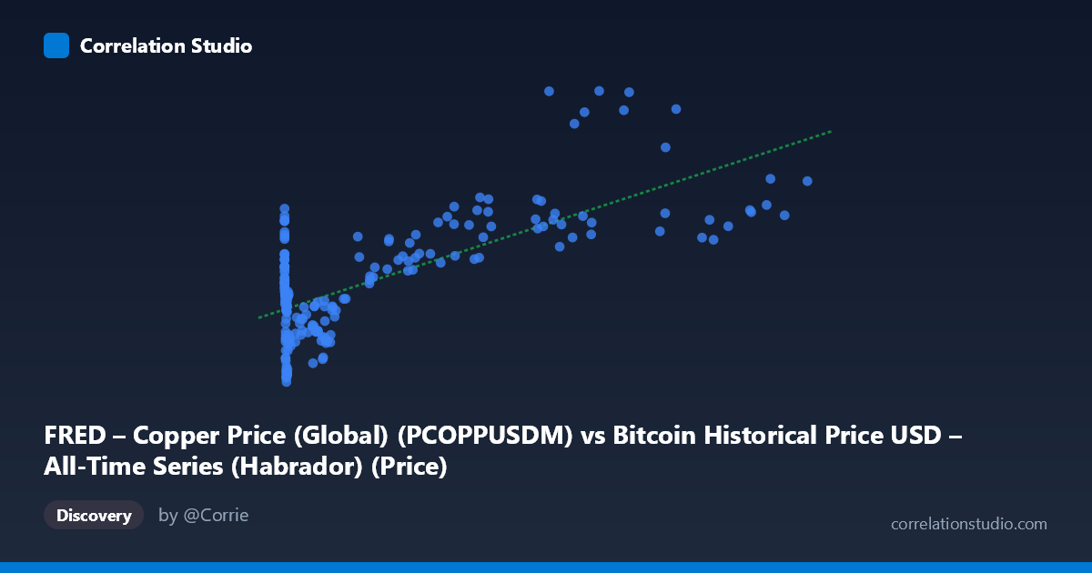
FRED – Copper Price (Global) (PCOPPUSDM) vs Bitcoin Historical Price USD – All-Time Series (Habrador) (Price)
- Pearson correlation (r)
- 0.7036
- Spearman correlation
- 0.4394
- p-value
- 0
- Sample size (n)
- 189
- 95% confidence interval
- 0.6235 to 0.7691
- Granger causality
- None
- Granger optimal lag
- 10
AI analysis
Analysis: Copper Price vs. Bitcoin Price
1. Relationship Overview
The scatterplot depicts a positive, moderately strong relationship between copper prices (X) and Bitcoin prices (Y), though the data structure is highly asymmetric. The X variable spans an enormous range (0.06 to 118,670 — note this range is implausible for copper prices in USD/tonne, suggesting a possible axis mislabeling or unit scaling issue) with extreme right-skew (mean 20,280 vs. median likely much lower, stdev nearly 30,000). Y (Bitcoin price, similarly mislabeled) ranges more modestly from ~4,472 to ~12,987. The bulk of observations cluster at low X values (under 1,000), while a sparse tail of high-X points extends the range dramatically, giving the scatter a classic "hockey stick" or logarithmic curve appearance rather than a clean linear cloud.
2. Strength, Direction, and Predictive Direction
The correlation coefficient (r = 0.70) indicates a moderately strong positive linear relationship, with r² = 0.49 meaning only about 49% of the variance in Y is explained by X — leaving over half unexplained by this single linear relationship. The 95% CI [0.619, 0.766] is reasonably tight and excludes zero, and the p-value (effectively 0) confirms this correlation is statistically robust and not due to chance, given n=188. However, statistical significance should not be conflated with practical predictive strength — r² of 0.49 leaves substantial room for other drivers.
The Granger causality results add a temporal dimension: X→Y is significant (F=2.60, p=0.006) at a 10-period lag, while Y→X is not (p=0.146). This suggests a unidirectional predictive relationship, where past values of X help forecast future Y beyond Y's own history, but not vice versa. This is consistent with a lagged, cumulative macro-driver relationship rather than simple contemporaneous co-movement — though Granger causality tests statistical precedence, not true causal mechanism.
3. Notable Patterns and Outliers
The data shows a clear non-linear, concave (log-like) shape: at low X values (0–1,000), Y varies substantially (4,600–9,600), indicating high noise/variance in this dense cluster. As X increases past ~10,000, Y rises more smoothly toward 9,000–10,700, suggesting the relationship may be better modeled logarithmically than linearly. Two notable outliers stand out: (77013, 12951) and (65792, 12529) — both with unusually high Y values relative to neighboring X values, breaking the otherwise smoother upper trend and likely exerting outsized leverage on the r² estimate. The linear fit (y = 0.0406x + 6745) will underfit the low-X cluster and may not capture curvature at the high end.
4. Confounding Factors and Caveats
Both variables are described as time series with 2010–2026 coverage, meaning this is almost certainly a spurious or confounded correlation driven by shared temporal/macro trends (both assets could be responding to global liquidity, USD strength, inflation expectations, or the same commodity supercycle) rather than a direct causal link between copper and Bitcoin. The mismatched axis descriptions (X labeled as Bitcoin history, Y labeled as copper) suggest a labeling error in the source data that should be resolved before drawing firm conclusions. Additionally, unequally spaced/sparse sampling at high X values means the tail is under-represented, and autocorrelation within each time series (common in financial data) can inflate apparent correlation and distort Granger test validity.
5. Recommendations
Given the labeling ambiguity, first verify which variable is genuinely copper and which is Bitcoin. Given the strong right-skew, refit using log-transformed X (and possibly Y) to test whether a log-linear model substantially improves r² and better represents the low-X cluster. Test for spurious correlation via a shared trend (detrend both series or use returns/differences rather than levels) and re-run Granger causality on stationary series to validate the lag-10 finding. Finally, isolate and investigate the two high-Y outliers (65,792/77,013 range) to determine if they correspond to a specific market event (e.g., 2021 speculative bull run) that may be distorting the overall fit.
X dataset: Bitcoin Historical Price USD – All-Time Series (Habrador)
Y dataset: FRED – Copper Price (Global)
Part of experiment: Bitcoin - Bitcoin Historical Price USD – All-Time Series (Habrador) vs FRED – Copper Price (Global)