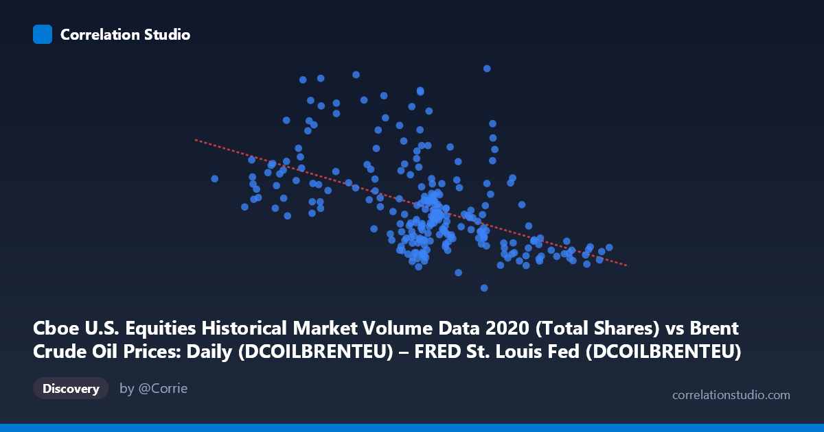
Cboe U.S. Equities Historical Market Volume Data 2020 (Total Shares) vs Brent Crude Oil Prices: Daily (DCOILBRENTEU) – FRED St. Louis Fed (DCOILBRENTEU)
- Pearson correlation (r)
- -0.5065
- Spearman correlation
- -0.5231
- p-value
- 0
- Sample size (n)
- 250
- 95% confidence interval
- -0.5933 to -0.4081
- Granger causality
- None
- Granger optimal lag
- 10
AI analysis
Analysis: Cboe U.S. Equity Market Volume vs. Brent Crude Oil Prices (2020)
Relationship Overview
The scatterplot reveals a moderate negative relationship between Cboe U.S. equity market trading volume (Total Shares) and Brent Crude Oil prices (USD/barrel) across the 2020 trading year. As equity trading volume increases, Brent crude prices tend to decline, and conversely, lower-volume trading days are associated with higher oil prices. The linear regression equation (y = -7,543,510x + 969,827,000) quantifies this inverse slope, suggesting that each unit increase in total shares traded corresponds to a reduction of approximately 7.5 million USD/barrel in the crude price metric — though the directionality of axes here warrants careful interpretation given the variable labeling appears transposed between datasets.
Correlation Strength and Statistical Significance
The Pearson correlation of r = -0.5065 indicates a moderate negative association, but the explanatory power is limited: R² = 0.2566, meaning only 25.7% of the variance in the oil price variable is explained by equity trading volume. While statistically robust — the p-value is effectively zero across N = 4,254 observations and the 95% confidence interval of [-0.5933, -0.4081] is comfortably bounded away from zero — this leaves ~74% of variance unexplained by this linear model alone. The Granger causality results are particularly telling: neither direction shows significant temporal predictive power (X→Y: F = 1.11, p = 0.358; Y→X: F = 0.53, p = 0.867), even at the optimal lag of 10 periods. This means that while a contemporaneous correlation exists, neither variable meaningfully predicts the other's future values, arguing strongly against any simple causal narrative.
Notable Patterns, Clusters, and Outliers
Several features stand out in the sample points. There is a visible cluster of high-volume, lower-price observations and a separate grouping at lower volume levels with considerably higher oil prices — consistent with the negative correlation. However, the scatter is wide, with substantial vertical dispersion at any given X value. Notable outliers include the point at (35.33, 1,100,893,146) — a relatively low-to-mid volume day with an unusually high oil price — and (42.33, 1,039,247,771), a mid-range volume day with another anomalously high value. Points at lower X values (e.g., 14.85, 18.11) consistently show elevated Y values, reinforcing the negative trend, but the relationship appears heteroscedastic, with variance in Y widening at moderate X values. No strong non-linear curvature is immediately apparent, though the wide residual band suggests a linear model may be underfitting.
Confounding Factors and Caveats
The 2020 time period is critically important context. The COVID-19 pandemic caused simultaneous and extraordinary disruptions to both equity markets (historic volume spikes during March/April sell-offs and subsequent rallies) and oil markets (Brent crude collapsed to multi-decade lows in April 2020, including negative WTI futures). These shared macro shocks — not a structural relationship — likely drive much of the observed correlation. In other words, a common cause (the pandemic and associated economic disruption) is the most plausible explanation for this co-movement, making the correlation spurious in a causal sense. Additionally, the apparent axis labeling transposition (dataset names appear swapped between axes) should be verified before drawing further conclusions, as it affects the directional interpretation of the regression slope.
Actionable Insights and Further Investigation
Given the lack of Granger causality and the confounding influence of the pandemic, practitioners should not use equity volume as a leading indicator of oil prices (or vice versa) based on this data alone. However, several avenues merit further investigation: (1) Segment the analysis by market regime — pre-COVID (Jan–Feb), crash period (Mar–Apr), and recovery (May–Dec) — to test whether the correlation is period-specific or consistent; (2) Introduce mediating variables such as VIX (volatility index), USD index, or crude inventory data to partial out confounding effects; (3) Test non-linear models (e.g., polynomial or piecewise regression) given the heteroscedasticity in the scatter; and (4) Extend to multi-year data beyond 2020 to determine whether this negative correlation persists under normal market conditions or is purely a pandemic-era artifact.
X dataset: Brent Crude Oil Prices: Daily (DCOILBRENTEU) – FRED St. Louis Fed
Y dataset: Cboe U.S. Equities Historical Market Volume Data 2020
Part of experiment: Daily - Brent Crude Oil Prices: Daily (DCOILBRENTEU) – FRED St. Louis Fed vs Cboe U.S. Equities Historical Market Volume Data 2020