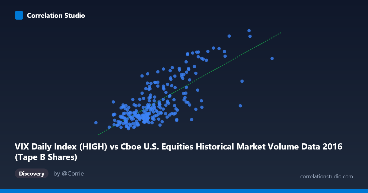
VIX Daily Index (HIGH) vs Cboe U.S. Equities Historical Market Volume Data 2016 (Tape B Shares)
- Pearson correlation (r)
- 0.7469
- Spearman correlation
- 0.685
- p-value
- 0
- Sample size (n)
- 252
- 95% confidence interval
- 0.6867 to 0.7969
- Granger causality
- None
- Granger optimal lag
- 1
AI analysis
Scatterplot Analysis: VIX High vs. Tape B Shares (2016)
Relationship Overview The scatterplot reveals a moderately strong positive relationship between the CBOE Volatility Index daily high (VIX) and Tape B share volume in U.S. equities markets during 2016. As VIX readings increase, Tape B trading volume rises in a broadly consistent pattern, which aligns with well-established market intuition: heightened uncertainty and fear (as measured by VIX) tends to drive increased trading activity across equity markets. The linear regression equation (y = 1.09e-07x + 5.21) captures this upward slope, though considerable scatter around the fitted line suggests the relationship is real but far from deterministic.
Correlation Strength and Statistical Interpretation With r = 0.747 and r² = 0.558, roughly 55.8% of the variance in Tape B share volume is explained by VIX highs, leaving approximately 44% attributable to other factors. The 95% confidence interval for r [0.687, 0.797] is reasonably tight and does not approach zero, and the p-value of effectively 0 (across n = 252 paired observations drawn from a population of 3,622) confirms this correlation is highly unlikely to be a chance finding. However, the Granger causality results complicate the narrative considerably: neither direction shows significant predictive causality (X→Y: F = 0.001, p = 0.974; Y→X: F = 0.197, p = 0.658). This means that while the two variables move together contemporaneously, neither reliably precedes or predicts the other temporally at a one-period lag — suggesting co-movement driven by shared underlying forces rather than a lead-lag relationship.
Notable Patterns, Clusters, and Outliers The sample points reveal a concentration of observations in the lower-left region of the chart (VIX ~60–100M range, Tape B ~12–18), consistent with the relatively calm market conditions that dominated much of 2016. A smaller but visually distinct cluster of high-VIX, high-volume points (e.g., VIX ~170M with Tape B ~28.43, and ~142M with ~27.22) likely corresponds to specific volatility events — most plausibly the Brexit vote (June 2016) and the U.S. presidential election (November 2016). These outlier observations may be disproportionately influencing the correlation coefficient, and their removal could meaningfully reduce r. The scatter also widens at higher X values, hinting at heteroscedasticity — variance in Tape B volume appears to increase as VIX rises, which violates a key assumption of ordinary least squares regression.
Confounding Factors and Caveats Several important caveats apply. First, both VIX levels and equity trading volumes are jointly driven by macro events (geopolitical shocks, monetary policy announcements, earnings seasons), making it difficult to isolate a direct mechanism between these two specific variables. Second, Tape B specifically covers NYSE American and regional exchange listings — a subset of total market activity — so its behavior may reflect idiosyncratic exchange routing dynamics rather than broad market responses to volatility. Third, the zero Granger causality finding at lag-1 suggests caution about treating this as any kind of predictive signal; the correlation may be entirely coincident within the same trading day. Finally, 2016 was an unusual year with discrete, identifiable shock events, and these findings may not generalize to other calendar years.
Actionable Insights and Further Investigation Practitioners should treat this correlation as contextually informative but not operationally predictive in its current form. Several follow-on analyses would strengthen understanding: (1) Test for heteroscedasticity formally (e.g., Breusch-Pagan test) and consider log-transforming both variables to stabilize variance; (2) Extend the Granger causality analysis to multiple lags (2–5 periods) to rule out slightly longer lead-lag dynamics; (3) Isolate the impact of the two or three major volatility events by running the correlation with and without those observations to assess their leverage on r²; (4) Compare this relationship across multiple years to assess whether 2016's event-driven structure is representative or anomalous; and (5) Incorporate additional explanatory variables (e.g., S&P 500 returns, bid-ask spreads, options expiry calendars) in a multivariate framework to better account for the remaining ~44% of unexplained variance.
X dataset: Cboe U.S. Equities Historical Market Volume Data 2016
Y dataset: VIX Daily Index
Part of experiment: Daily - Cboe U.S. Equities Historical Market Volume Data 2016 vs VIX Daily Index