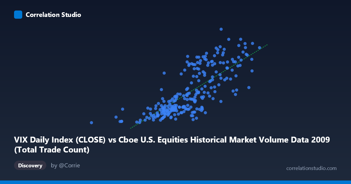
VIX Daily Index (CLOSE) vs Cboe U.S. Equities Historical Market Volume Data 2009 (Total Trade Count)

Pearson correlation (r): 0.7698
Spearman correlation: 0.8005
p-value: 0
Sample size (n): 252
95% confidence interval: 0.7141 to 0.8158
Granger causality: None
Granger optimal lag: 1

AI analysis

VIX vs. Total Trade Count: Correlation Analysis (2009)

Overview of the Relationship

The scatterplot reveals a moderately strong positive relationship between the CBOE VIX Daily Index closing values and the total trade count in U.S. equities markets during 2009. As VIX levels rise — indicating greater market fear and uncertainty — trading activity (measured by total trade count) tends to increase meaningfully. This aligns intuitively with well-established market microstructure theory: elevated volatility regimes drive increased portfolio rebalancing, hedging activity, stop-loss executions, and speculative positioning, all of which generate more discrete trades. The data spans the full calendar year 2009, a period of exceptional market stress following the 2008 financial crisis, making it a particularly rich environment to observe this dynamic.

Correlation Strength, Direction, and Statistical Significance

The Pearson correlation of r = 0.7698 indicates a strong positive association, and the R² of 0.5926 means that approximately 59.3% of the variance in trade count is explained by VIX levels — a substantial but incomplete explanatory relationship. The remaining ~40.7% of variance reflects other drivers not captured by VIX alone. The 95% confidence interval of [0.7141, 0.8158] is notably tight, reflecting the large paired sample size of n = 252, and the p-value of essentially zero confirms this result is highly statistically significant and extremely unlikely to be due to chance. The linear regression equation (y = 1.1668×10⁻⁵x + 0.360) suggests that each unit increase in VIX is associated with a meaningful incremental rise in trade count. However, despite the strong contemporaneous correlation, Granger causality tests found no significant predictive directionality in either direction (X→Y: F = 0.29, p = 0.59; Y→X: F = 0.07, p = 0.80). This is a critical nuance — while VIX and trade count move together, neither variable reliably predicts the other at a one-period lag, suggesting the relationship is likely contemporaneous and driven by shared underlying conditions rather than a leading/lagging causal mechanism.

Notable Patterns, Clusters, and Outliers

The scatterplot exhibits several visually distinct features. There appears to be a dense cluster in the lower-left region — corresponding to VIX values roughly in the 20–30 range and lower trade counts — which likely represents the calmer second half of 2009 as markets stabilized post-crisis lows in March. A secondary, more dispersed cluster emerges at higher VIX values (35–55), associated with elevated trade counts, likely corresponding to the volatile early 2009 period. The extreme point near (629671.25, 19.47) stands out as a potential outlier with a very low X value (trade count) paired with a low VIX reading, possibly reflecting a data anomaly or a holiday-shortened trading session with atypically thin volume. Similarly, several points at the upper range of VIX (approaching 56) show high trade counts but with notable scatter, suggesting heteroscedasticity — variance in trade count increases at higher VIX levels, which is consistent with the less predictable nature of panic-driven markets.

Confounding Factors and Interpretive Caveats

Several important caveats apply. First, 2009 is not a typical year — it spans the tail of the financial crisis and a historic market recovery, meaning the range of VIX values observed (nearly 20 to 57) is far wider than in normal years, which artificially inflates the apparent correlation. Second, secular trends in electronic trading and market fragmentation were accelerating during this period, meaning trade counts were rising independently of volatility due to structural market changes (e.g., growth of high-frequency trading). This could induce spurious correlation if both variables were simultaneously trending. Third, the axes appear to have been swapped in dataset labeling — VIX data is described under the "Market Volume" dataset column and vice versa, which warrants verification before any downstream use. Fourth, the absence of Granger causality may partially reflect the coarseness of the one-period lag tested; intraday or multi-lag analysis might reveal different temporal dynamics.

Actionable Insights and Further Investigation

Practitioners could use this relationship as a regime indicator: when VIX exceeds certain thresholds (e.g., 35–40), market infrastructure, liquidity providers, and exchanges should anticipate significantly elevated trade volumes and ensure operational capacity accordingly. For further investigation, it would be valuable to: (1) test non-linear model fits (e.g., logarithmic or polynomial), given the apparent heteroscedasticity and possible diminishing returns at extreme VIX levels; (2) disaggregate by exchange venue to determine whether the VIX–volume relationship is uniform across all U.S. equity venues or concentrated in specific markets; (3) extend the analysis to multiple years to test whether 2009's crisis-era dynamics are representative or exceptional; and (4) incorporate additional explanatory variables such as S&P 500 returns, bid-ask spreads, or market depth metrics to build a more complete model of what drives the remaining ~41% of unexplained variance.

X dataset: Cboe U.S. Equities Historical Market Volume Data 2009

Y dataset: VIX Daily Index

Part of experiment: Daily - Cboe U.S. Equities Historical Market Volume Data 2009 vs VIX Daily Index